图像小波变换与多分辨率
小波变换是近年来图像处理领域备受关注的新技术,尤其在图像压缩、特征检测和纹理分析等方面展现出巨大潜力。它通过多分辨率分析、时频域分析和金字塔算法等方法,为图像处理提供了全新的视角。
从傅里叶变换到小波变换
小波的概念
小波是在有限时间范围内变化且平均值为0的数学函数,具有有限持续时间和突变的频率与振幅两大特点。小波变换通过平移和缩放母小波,捕获信号的时间和频域信息,其结果为各种小波系数,反映局部信号与小波的相关程度。
感性认识小波变换
傅里叶变换是信号处理领域的经典分析手段,实现时域与频域的相互转化,但其无法提供信号在局部时间段的频率信息。例如,两个在时域上差异显著的信号,在频域上可能非常相似。
python
import numpy as np
import matplotlib.pyplot as plt
from scipy.fftpack import fft

# 中文显示工具函数
def set_ch():
    from pylab import mpl
    mpl.rcParams['font.sans-serif'] = ['FangSong']
    mpl.rcParams['axes.unicode_minus'] = False

set_ch()
t = np.linspace(0, 1, 400, endpoint=False)
cond = [t < 0.25, (t >= 0.25) & (t < 0.5), t >= 0.5]
f1 = lambda t: np.cos(2 * np.pi * 10 * t)
f2 = lambda t: np.cos(2 * np.pi * 50 * t)
f3 = lambda t: np.cos(2 * np.pi * 100 * t)
y1 = np.piecewise(t, cond, [f1, f2, f3])
y2 = np.piecewise(t, cond, [f2, f1, f3])
Y1 = abs(fft(y1))
Y2 = abs(fft(y2))

plt.figure(figsize=(12, 9))

plt.subplot(221)
plt.plot(t, y1)
plt.title('信号1 时间域')
plt.xlabel('时间/s')

plt.subplot(222)
plt.plot(range(400), Y1)
plt.title('信号1 频率域')
plt.xlabel('频率/Hz')

plt.subplot(223)
plt.plot(t, y2)
plt.title('信号2 时间域')
plt.xlabel('时间/s')

plt.subplot(224)
plt.plot(range(400), Y2)
plt.title('信号2 频率域')
plt.xlabel('频率/Hz')

plt.show()
为解决这一问题,可以采用加窗的短时距傅里叶变换,将长时间信号分割成多个较短的等长信号,再分别进行傅里叶变换,从而得到频率随时间的变化情况。
python
import numpy as np
import matplotlib.pyplot as plt
import pywt
# 中文显示工具函数
def set_ch():
from pylab import mpl
mpl.rcParams['font.sans-serif'] = ['FangSong']
mpl.rcParams['axes.unicode_minus'] = False
set_ch()
t = np.linspace(0, 1, 400, endpoint=False)
cond = [t < 0.25, (t >= 0.25) & (t < 0.5), t >= 0.5]
f1 = lambda t: np.cos(2 * np.pi * 10 * t)
f2 = lambda t: np.cos(2 * np.pi * 50 * t)
f3 = lambda t: np.cos(2 * np.pi * 100 * t)
y1 = np.piecewise(t, cond, [f1, f2, f3])
y2 = np.piecewise(t, cond, [f2, f1, f3])
cwtmatr1, freqs1 = pywt.cwt(y1, np.arange(1, 200), 'cgau8', 1 / 400)
cwtmatr2, freqs2 = pywt.cwt(y2, np.arange(1, 200), 'cgau8', 1 / 400)
plt.figure(figsize=(12, 9))
plt.subplot(221)
plt.plot(t, y1)
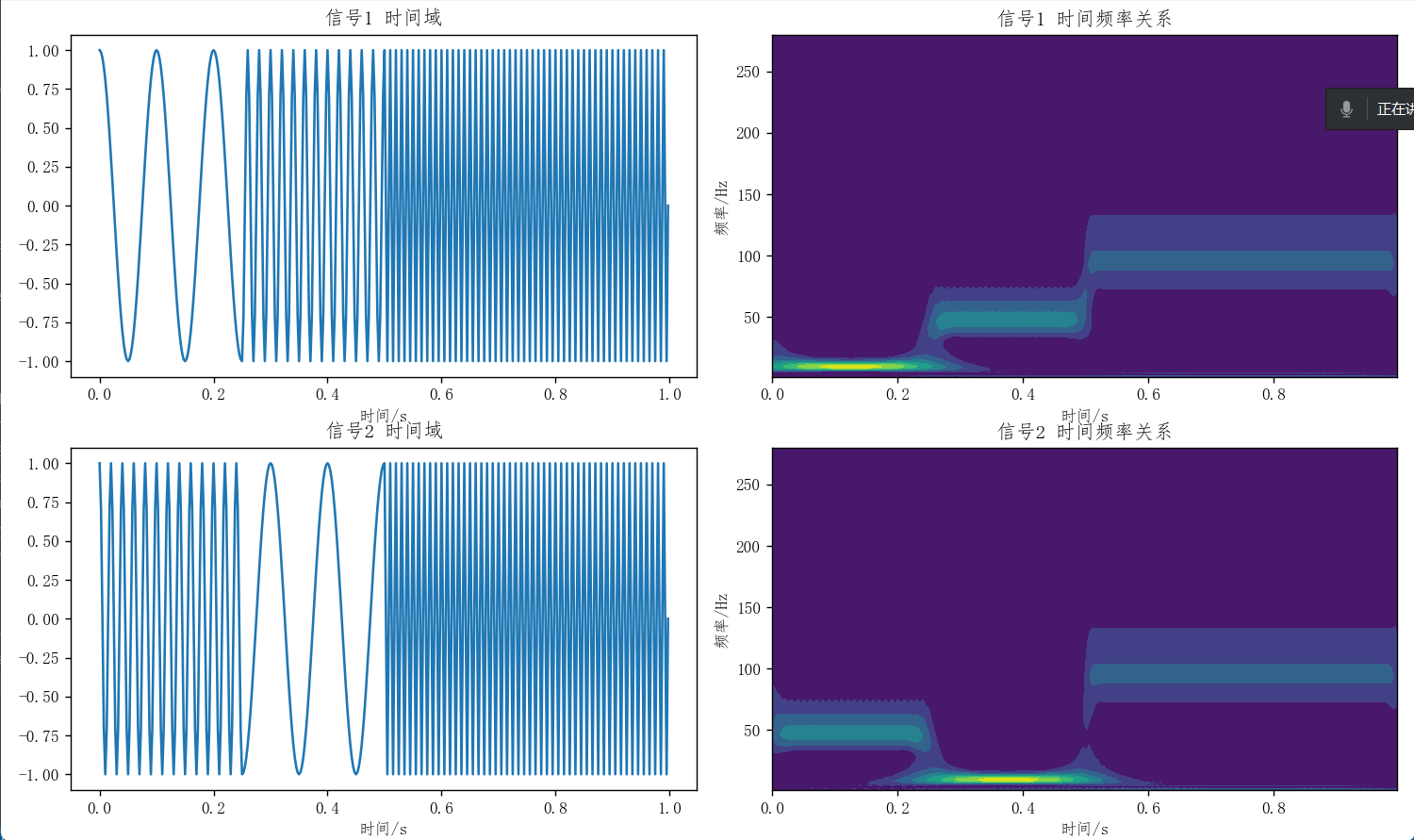
plt.title('信号1 时间域')
plt.xlabel('时间/s')
plt.subplot(222)
plt.contourf(t, freqs1, abs(cwtmatr1))
plt.title('信号1 时间频率关系')
plt.xlabel('时间/s')
plt.ylabel('频率/Hz')
plt.subplot(223)
plt.plot(t, y2)
plt.title('信号2 时间域')
plt.xlabel('时间/s')
plt.subplot(224)
plt.contourf(t, freqs2, abs(cwtmatr2))
plt.title('信号2 时间频率关系')
plt.xlabel('时间/s')
plt.ylabel('频率/Hz')
plt.tight_layout()
plt.show()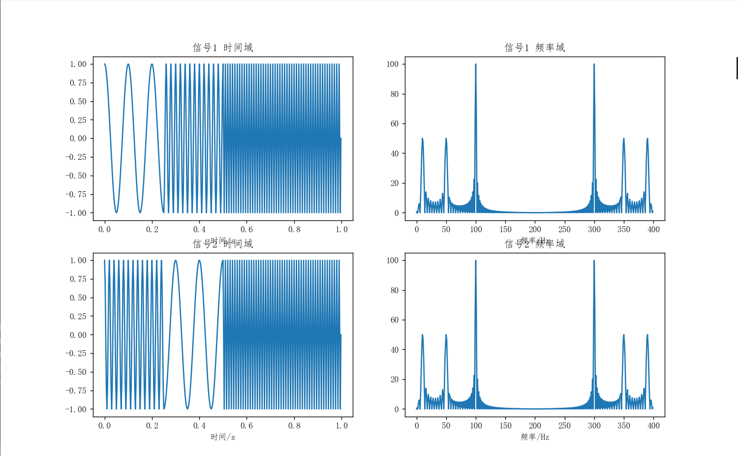
小波变换则能同时提供信号的频率和时间信息,弥补了傅里叶变换的不足。它不仅知道信号中有哪些成分,还能知道这些成分在什么位置出现。
简单小波示例
哈尔小波构建
哈尔小波具有以下特点:
- 在时域是紧支撑的,非零区间为[0,1)
- 属于正交小波
- 具有对称性,系统单位冲击响应对称,有利于去除相位失真
- 仅取+1和-1,计算简单
- 是不连续小波,在实际信号分析与处理中存在一定限制
图像多分辨率
小波多分辨率
多分辨分析是小波分析的核心概念之一,将函数表示为低频成分与不同分辨率下的高频成分,具备以下特性:
- 单调性
- 伸缩性
- 平移不变性
- Riesz基
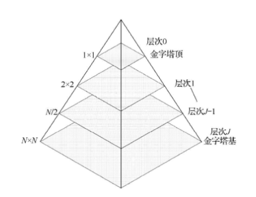
图像金字塔
图像金字塔用于机器视觉或图像压缩,将图像表示为一系列分辨率逐渐降低的集合。多分辨率分析中,每层包含一个近似图像和一个残差图像,多种分辨率层次联合形成图像金字塔。
图像子带编码
子带编码将图像分解为多个频带受限的分量,称为子带。子带可重组无失真重建原始图像,每个子带通过带通滤波输入图像获得。
图像小波变换
二维小波变换基础
二维离散小波变换输入二维矩阵,每个步骤输出近似图像、水平细节、垂直细节和对角细节。
python
import numpy as np
import matplotlib.pyplot as plt
import pywt.data

# 中文显示工具函数
def set_ch():
    from pylab import mpl
    mpl.rcParams['font.sans-serif'] = ['FangSong']
    mpl.rcParams['axes.unicode_minus'] = False

set_ch()
original = pywt.data.camera()
# Wavelet transform of image, and plot approximation and details
titles = ['近似图像', '水平细节', '垂直细节', '对角线细节']
coeffs2 = pywt.dwt2(original, 'haar')
LL, (LH, HL, HH) = coeffs2
fig = plt.figure(figsize=(12, 3))
for i, a in enumerate([LL, LH, HL, HH]):
    ax = fig.add_subplot(1, 4, i + 1)
    ax.imshow(a, interpolation="nearest", cmap=plt.cm.gray)
    ax.set_title(titles[i], fontsize=10)
    ax.set_xticks([])
    ax.set_yticks([])
fig.tight_layout()
plt.show()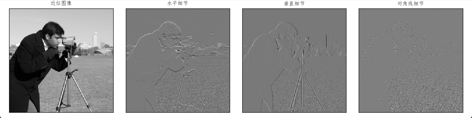
小波变换在图像处理中的应用
小波变换在图像处理中的应用步骤:
- 计算图像的二维小波变换,得到小波系数
- 修改小波系数,保留有效成分,过滤不必要成分
- 使用修改后的小波系数重建图像
基于小波变换的图像去噪
python
import numpy as np
import matplotlib.pyplot as plt
import pywt
from skimage.restoration import denoise_wavelet

# 中文显示工具函数
def set_ch():
    from pylab import mpl
    mpl.rcParams['font.sans-serif'] = ['FangSong']
    mpl.rcParams['axes.unicode_minus'] = False

set_ch()
x = pywt.data.ecg().astype(float) / 256

sigma = .05
x_noisy = x + sigma * np.random.randn(x.size)
x_denoise = denoise_wavelet(x_noisy, sigma=sigma, wavelet='sym4')

plt.subplot(311)
plt.title('原始信号')
plt.plot(x)

plt.subplot(312)
plt.title('加噪图像')
plt.plot(x_noisy)

plt.subplot(313)
plt.title('去噪图像')
plt.plot(x_denoise)

plt.show()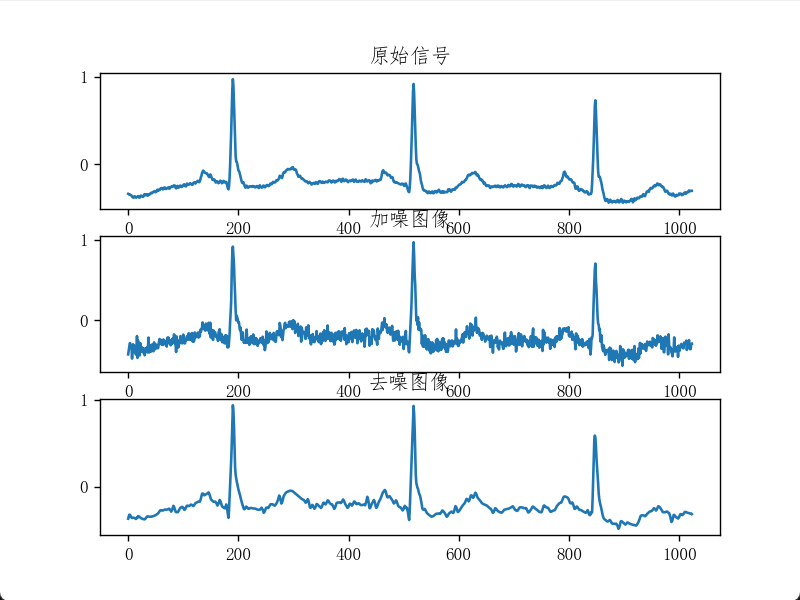
python
import matplotlib.pyplot as plt
from skimage.restoration import (denoise_wavelet, estimate_sigma)
from skimage import data, img_as_float
from skimage.util import random_noise
# 中文显示工具函数
def set_ch():
from pylab import mpl
mpl.rcParams['font.sans-serif'] = ['FangSong']
mpl.rcParams['axes.unicode_minus'] = False
set_ch()
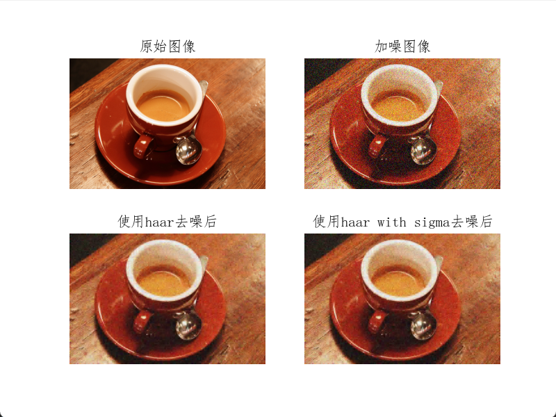
original = img_as_float(data.coffee())
plt.subplot(221)
plt.axis('off')
plt.title('原始图像')
plt.imshow(original)
sigma = 0.2
noisy = random_noise(original, var=sigma ** 2)
plt.subplot(222)
plt.axis('off')
plt.title('加噪图像')
plt.imshow(noisy)
im_haar = denoise_wavelet(noisy, wavelet='db2', channel_axis=-1, convert2ycbcr=True)
plt.subplot(223)
plt.axis('off')
plt.title('使用haar去噪后')
plt.imshow(im_haar)
# 不同颜色通道的噪声平均标准差
sigma_est = estimate_sigma(noisy, channel_axis=-1, average_sigmas=True)
im_haar_sigma = denoise_wavelet(noisy, wavelet='db2', channel_axis=-1, convert2ycbcr=True, sigma=sigma_est)
plt.subplot(224)
plt.axis('off')
plt.title('使用haar with sigma去噪后')
plt.imshow(im_haar_sigma)
plt.show()