Image Wavelet Transform and Multi-resolution Analysis
Wavelet transform is a cutting-edge image processing technology that has garnered significant attention in recent years. It has spurred the development of numerous innovative methods in areas such as image compression, feature detection, and texture analysis, including multi-resolution analysis, time-frequency analysis, and pyramid algorithms, all of which fall under the wavelet transform umbrella.
From Fourier Transform to Wavelet Transform
Concept of Wavelets
A wavelet is a mathematical function that undergoes changes within a limited time frame and has an average value of zero. It possesses two key characteristics: (1) it has a finite duration with sudden changes in frequency and amplitude, and (2) within this limited time frame, its average value is zero. The result of a wavelet transform is various wavelet coefficients composed of scale and displacement functions.
Intuitive Understanding of Wavelet Transform
The Fourier transform has long been the most widely used and effective analysis tool in signal processing, serving as a means to convert between time and frequency domains. However, while the Fourier transform can provide frequency information across the entire time domain, it fails to offer frequency information for specific local time segments.
For instance, two signals that appear very different in the time domain may look quite similar in the frequency domain when analyzed using the Fourier transform.
import numpy as np
import matplotlib.pyplot as plt
from scipy.fftpack import fft

# Function for Chinese font display
def set_ch():
    from pylab import mpl
    mpl.rcParams['font.sans-serif'] = ['FangSong']
    mpl.rcParams['axes.unicode_minus'] = False

set_ch()
t = np.linspace(0, 1, 400, endpoint=False)
cond = [t < 0.25, (t >= 0.25) & (t < 0.5), t >= 0.5]
f1 = lambda t: np.cos(2 * np.pi * 10 * t)
f2 = lambda t: np.cos(2 * np.pi * 50 * t)
f3 = lambda t: np.cos(2 * np.pi * 100 * t)
y1 = np.piecewise(t, cond, [f1, f2, f3])
y2 = np.piecewise(t, cond, [f2, f1, f3])
Y1 = abs(fft(y1))
Y2 = abs(fft(y2))

plt.figure(figsize=(12, 9))

plt.subplot(221)
plt.plot(t, y1)
plt.title('Signal 1 Time Domain')
plt.xlabel('Time/s')

plt.subplot(222)
plt.plot(range(400), Y1)
plt.title('Signal 1 Frequency Domain')
plt.xlabel('Frequency/Hz')

plt.subplot(223)
plt.plot(t, y2)
plt.title('Signal 2 Time Domain')
plt.xlabel('Time/s')

plt.subplot(224)
plt.plot(range(400), Y2)
plt.title('Signal 2 Frequency Domain')
plt.xlabel('Frequency/Hz')

plt.show()
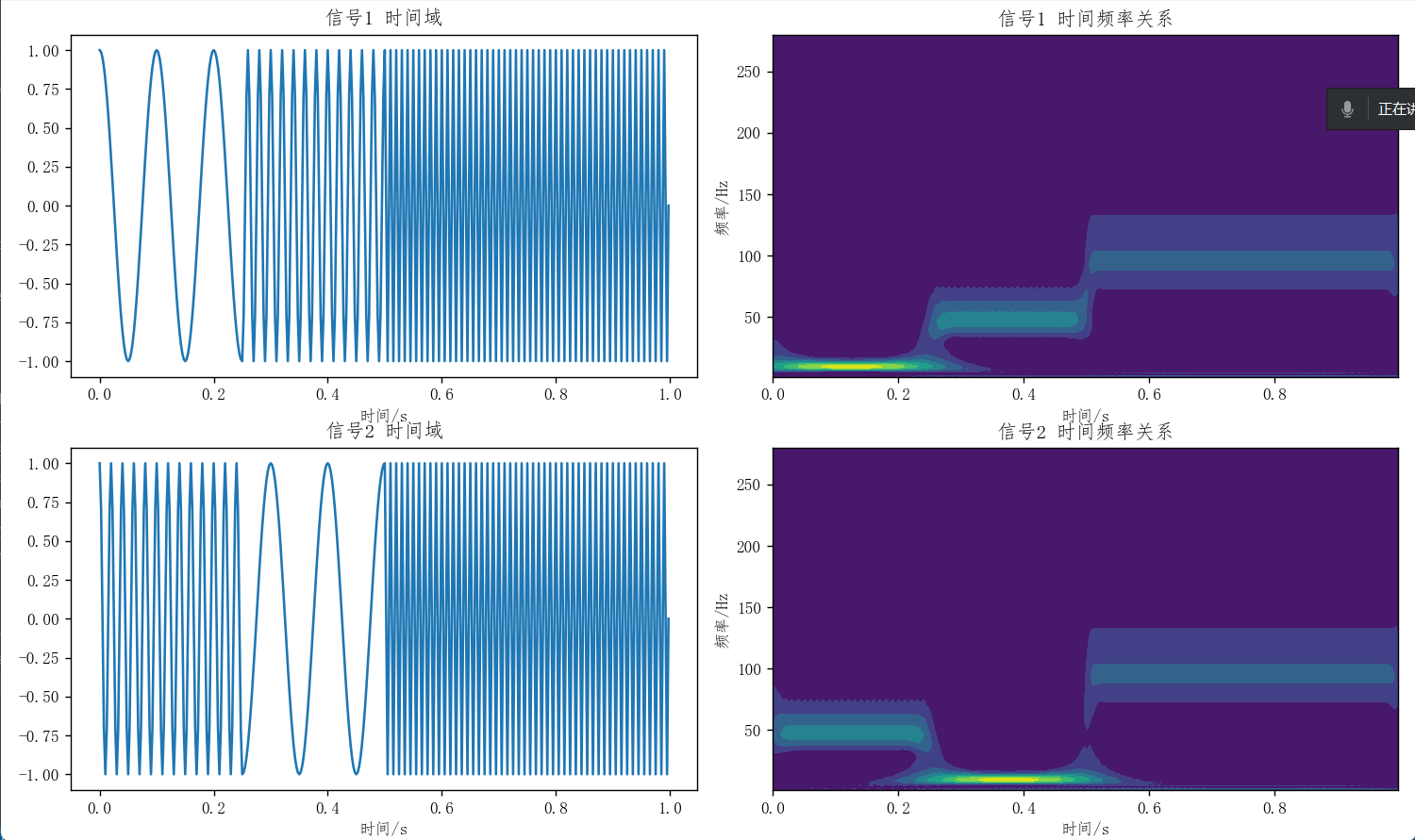
To address this limitation, windowing (Short-Time Fourier Transform) can be employed, dividing long-duration signals into shorter, equal-length segments and then performing Fourier transforms on each window to obtain frequency changes over time.
import numpy as np
import matplotlib.pyplot as plt
import pywt

# Function for Chinese font display
def set_ch():
    from pylab import mpl
    mpl.rcParams['font.sans-serif'] = ['FangSong']
    mpl.rcParams['axes.unicode_minus'] = False

set_ch()
t = np.linspace(0, 1, 400, endpoint=False)
cond = [t < 0.25, (t >= 0.25) & (t < 0.5), t >= 0.5]

f1 = lambda t: np.cos(2 * np.pi * 10 * t)
f2 = lambda t: np.cos(2 * np.pi * 50 * t)
f3 = lambda t: np.cos(2 * np.pi * 100 * t)

y1 = np.piecewise(t, cond, [f1, f2, f3])
y2 = np.piecewise(t, cond, [f2, f1, f3])

cwtmatr1, freqs1 = pywt.cwt(y1, np.arange(1, 200), 'cgau8', 1 / 400)
cwtmatr2, freqs2 = pywt.cwt(y2, np.arange(1, 200), 'cgau8', 1 / 400)

plt.figure(figsize=(12, 9))

plt.subplot(221)
plt.plot(t, y1)
plt.title('Signal 1 Time Domain')
plt.xlabel('Time/s')

plt.subplot(222)
plt.contourf(t, freqs1, abs(cwtmatr1))
plt.title('Signal 1 Time-Frequency Relationship')
plt.xlabel('Time/s')
plt.ylabel('Frequency/Hz')

plt.subplot(223)
plt.plot(t, y2)
plt.title('Signal 2 Time Domain')
plt.xlabel('Time/s')

plt.subplot(224)
plt.contourf(t, freqs2, abs(cwtmatr2))
plt.title('Signal 2 Time-Frequency Relationship')
plt.xlabel('Time/s')
plt.ylabel('Frequency/Hz')

plt.tight_layout()
plt.show()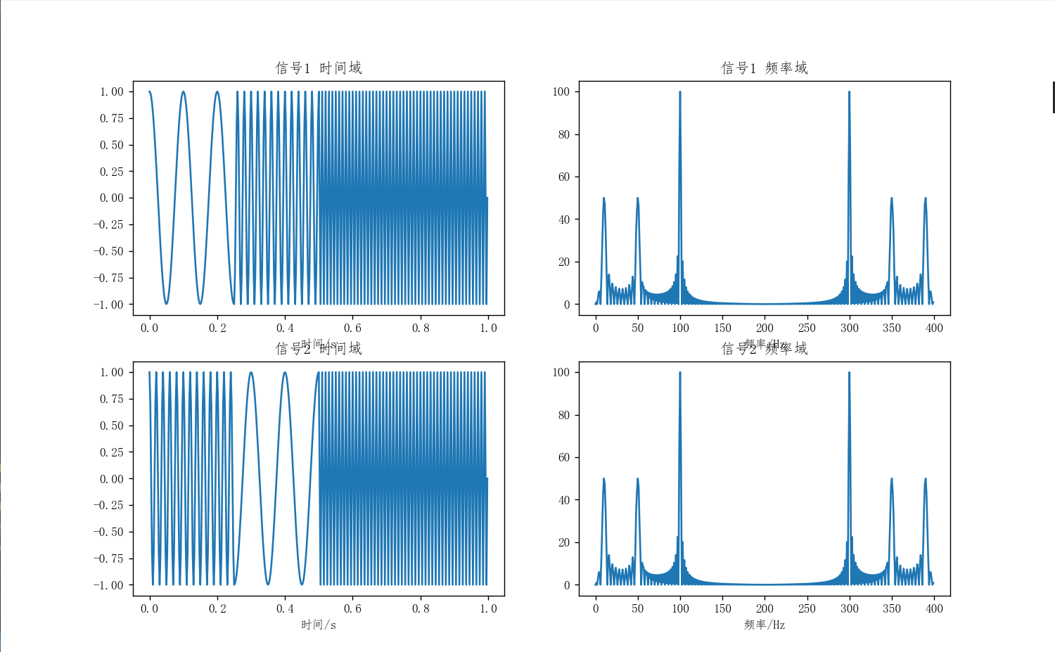
Wavelet transform overcomes the limitations of Fourier transform by providing both time and frequency information. It can identify not only the frequency components of a signal but also when these components occur.
Simple Wavelet Examples
Haar Wavelet Construction
The Haar wavelet has the following characteristics:
- It is compactly supported in the time domain, with a non-zero interval of [0,1)
- It belongs to orthogonal wavelets
- It is symmetric, which helps eliminate phase distortion
- It takes only +1 and -1, making calculations simple
- It is a discontinuous wavelet with certain limitations in practical signal analysis and processing
Image Multi-resolution Analysis
Wavelet Multi-resolution
Multi-resolution analysis is a core concept in wavelet analysis. It represents a function as a combination of low-frequency components and high-frequency components at different resolutions. The properties of multi-resolution analysis include:
- Monotonicity
- Scalability
- Translation invariance
- Riesz basis
Image Pyramid
Image pyramids are used in machine vision or image compression, representing an image as a collection of gradually downsampled images. In multi-resolution analysis, each level contains an approximation image and a residual image, forming what is known as an image pyramid when combined across resolutions.
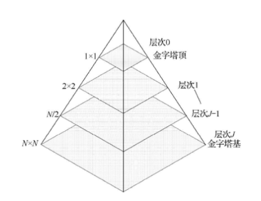
Image Subband Coding
In subband coding, an image is decomposed into multiple subbands, each of which is a frequency-band limited component. These subbands can be combined to reconstruct the original image without distortion, with each subband obtained by applying a bandpass filter to the input image.
Image Wavelet Transform
Fundamentals of 2D Wavelet Transform
The 2D discrete wavelet transform takes a 2D matrix as input. Each step produces an approximation image, horizontal details, vertical details, and diagonal details.
import numpy as np
import matplotlib.pyplot as plt
import pywt.data

# Function for Chinese font display
def set_ch():
    from pylab import mpl
    mpl.rcParams['font.sans-serif'] = ['FangSong']
    mpl.rcParams['axes.unicode_minus'] = False

set_ch()
original = pywt.data.camera()
# Wavelet transform of image, and plot approximation and details
titles = ['Approximation Image', 'Horizontal Details', 'Vertical Details', 'Diagonal Details']
coeffs2 = pywt.dwt2(original, 'haar')
LL, (LH, HL, HH) = coeffs2
fig = plt.figure(figsize=(12, 3))
for i, a in enumerate([LL, LH, HL, HH]):
    ax = fig.add_subplot(1, 4, i + 1)
    ax.imshow(a, interpolation="nearest", cmap=plt.cm.gray)
    ax.set_title(titles[i], fontsize=10)
    ax.set_xticks([])
    ax.set_yticks([])
fig.tight_layout()
plt.show()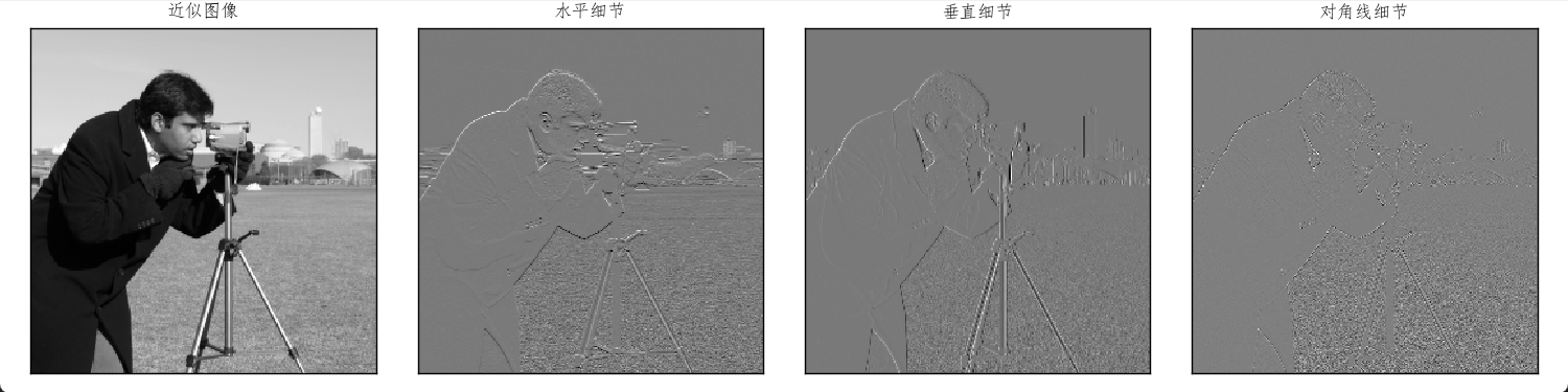
Applications of Wavelet Transform in Image Processing
The application of wavelet transform in image processing involves similar steps to Fourier transform:
- Compute the 2D wavelet transform of an image to obtain wavelet coefficients
- Modify the wavelet coefficients to retain effective components and filter out unnecessary ones
- Reconstruct the image using the modified wavelet coefficients
Image Denoising Using Wavelet Transform
import numpy as np
import matplotlib.pyplot as plt
import pywt
from skimage.restoration import denoise_wavelet

# Function for Chinese font display
def set_ch():
    from pylab import mpl
    mpl.rcParams['font.sans-serif'] = ['FangSong']
    mpl.rcParams['axes.unicode_minus'] = False

set_ch()
x = pywt.data.ecg().astype(float) / 256

sigma = .05
x_noisy = x + sigma * np.random.randn(x.size)
x_denoise = denoise_wavelet(x_noisy, sigma=sigma, wavelet='sym4')

plt.subplot(311)
plt.title('Original Signal')
plt.plot(x)

plt.subplot(312)
plt.title('Noisy Image')
plt.plot(x_noisy)

plt.subplot(313)
plt.title('Denoised Image')
plt.plot(x_denoise)

plt.show()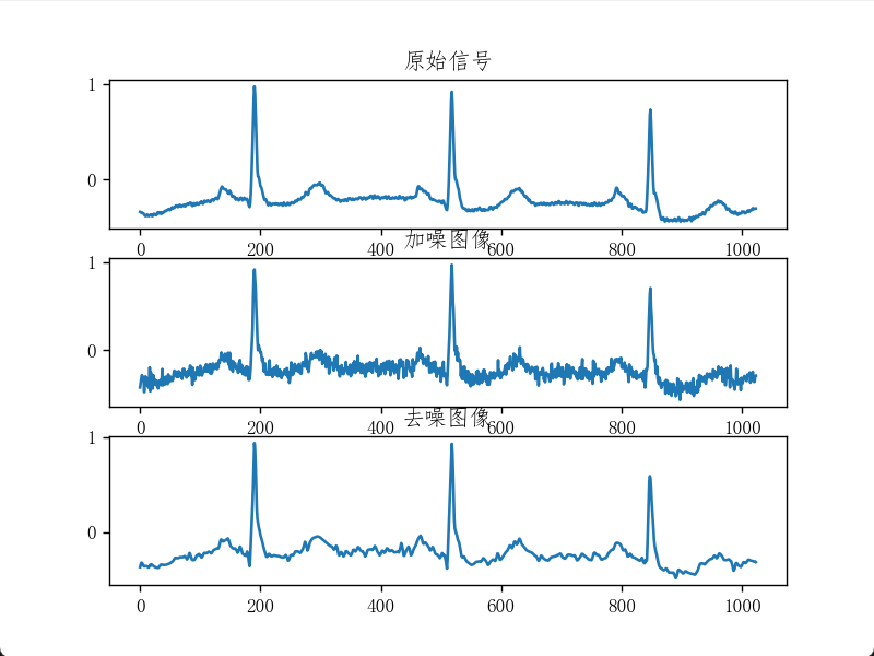
import matplotlib.pyplot as plt
from skimage.restoration import (denoise_wavelet, estimate_sigma)
from skimage import data, img_as_float
from skimage.util import random_noise
# Function for Chinese font display
def set_ch():
from pylab import mpl
mpl.rcParams['font.sans-serif'] = ['FangSong']
mpl.rcParams['axes.unicode_minus'] = False
set_ch()
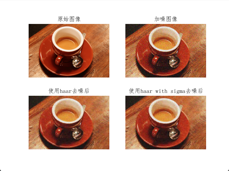
original = img_as_float(data.coffee())
plt.subplot(221)
plt.axis('off')
plt.title('Original Image')
plt.imshow(original)
sigma = 0.2
noisy = random_noise(original, var=sigma ** 2)
plt.subplot(222)
plt.axis('off')
plt.title('Noisy Image')
plt.imshow(noisy)
im_haar = denoise_wavelet(noisy, wavelet='db2', channel_axis=-1, convert2ycbcr=True)
plt.subplot(223)
plt.axis('off')
plt.title('Denoised with Haar')
plt.imshow(im_haar)
# Estimate the average noise standard deviation across color channels
sigma_est = estimate_sigma(noisy, channel_axis=-1, average_sigmas=True)
im_haar_sigma = denoise_wavelet(noisy, wavelet='db2', channel_axis=-1, convert2ycbcr=True, sigma=sigma_est)
plt.subplot(224)
plt.axis('off')
plt.title('Denoised with Haar and Sigma')
plt.imshow(im_haar_sigma)
plt.show()