Decision Tree

1. Overview of Decision Tree

The decision tree is a type of supervised machine learning. It has a very early origin, conforms to intuition and is highly intuitive. It imitates the human decision-making process. It was widely applied in early artificial intelligence models. Nowadays, some ensemble learning algorithms based on decision trees are more commonly used. If we thoroughly understand the decision tree algorithm in this chapter, it will be of great help for us to learn ensemble learning later.

1.1 Example 1

We have the following data:

ID	Own Real Estate (Yes/No)	Marital Status [Single, Married, Divorced]	Annual Income (in Thousands of Yuan)	Unable to Repay Debt (Yes/No)
1	Yes	Single	125	No
2	No	Married	100	No
3	No	Single	70	No
4	Yes	Married	120	No
5	No	Divorced	95	Yes
6	No	Married	60	No
7	Yes	Divorced	220	No
8	No	Single	85	Yes
9	No	Married	75	No
10	No	Single	90	Yes

The above table records whether existing users can repay debts according to historical data, as well as related information. Based on this data, the constructed decision tree is as follows:

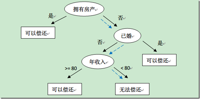
For example, if a new user comes: without real estate, single, with an annual income of 55K, then according to the above decision tree, it can be predicted that he cannot repay the debt (the blue dashed path). From the above decision tree, we can also know that whether a user owns real estate can greatly determine whether the user can repay the debt, which has guiding significance for the lending business.

1.2 Example 2

The girl's mother wants to introduce a blind date to her. When asked about the age, the mother says it's 24. Is he handsome? Quite handsome. Is his income high? He has a medium income. Is he a civil servant? The mother says yes. The girl: Okay, I'll go and meet him.

Construct a decision tree according to the case:

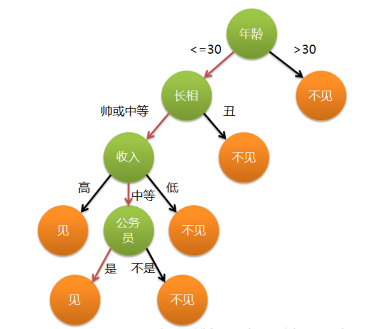
Question: Is the picture a binary tree?

The decision tree is a standard binary tree, and each node has only two branches~

• In the above tree, the attributes are the green nodes (Age, Appearance, Income, Whether to Be a Civil Servant)
  • The attributes are called data, generally represented by X.
  • Corresponding to the attributes, the target values (the orange nodes) are generally represented by y.
• When constructing this tree, the sequence varies for each person, and with different standards, the tree structures are different.
• When a computer constructs a tree, the standards are consistent, and the constructed trees are the same.

1.3 Characteristics of the Decision Tree Algorithm

• It can handle nonlinear problems.
• It has strong interpretability, and there are no equation coefficients $\theta$.
• The model is simple, and the model's prediction efficiency is high.

2. Usage of DecisionTreeClassifier

2.1 Introduction to the Example

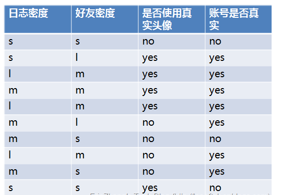
Among them, s, m, and l represent small, medium, and large respectively.

Whether the account is real is related to the attributes: Log Density, Friend Density, and Whether to Use a Real Avatar~

2.2 Construct and Visualize the Decision Tree

Data Creation

import numpy as np
import pandas as pd
y = np.array(list('NYYYYYNYYN'))
print(y)
X = pd.DataFrame({'Log Density':list('sslmlmmlms'),
                  'Friend Density':list('slmmmlsmss'),
                  'Real Avatar':list('NYYYYNYYYY'),
                  'Real User':y})
X

Model Training (An error occurs because the data type is a string)

from sklearn.tree import DecisionTreeClassifier

model = DecisionTreeClassifier()

model.fit(X,y)

Data Modification (Use the map function to perform data conversion)

X['Log Density'] = X['Log Density'].map({'s':0,'m':1,'l':2})
X['Friend Density'] = X['Friend Density'].map({'s':0,'m':1,'l':2})
X['Real Avatar'] = X['Real Avatar'].map({'N':0,'Y':1})
X

Model Training and Visualization

import matplotlib.pyplot as plt
# Use information entropy as the splitting criterion
model = DecisionTreeClassifier(criterion='entropy')
model.fit(X,y)
plt.rcParams['font.family'] = 'STKaiti'
plt.figure(figsize=(12,16))
fn = X.columns
_ = tree.plot_tree(model,filled = True,feature_names=fn)
plt.savefig('./iris.jpg')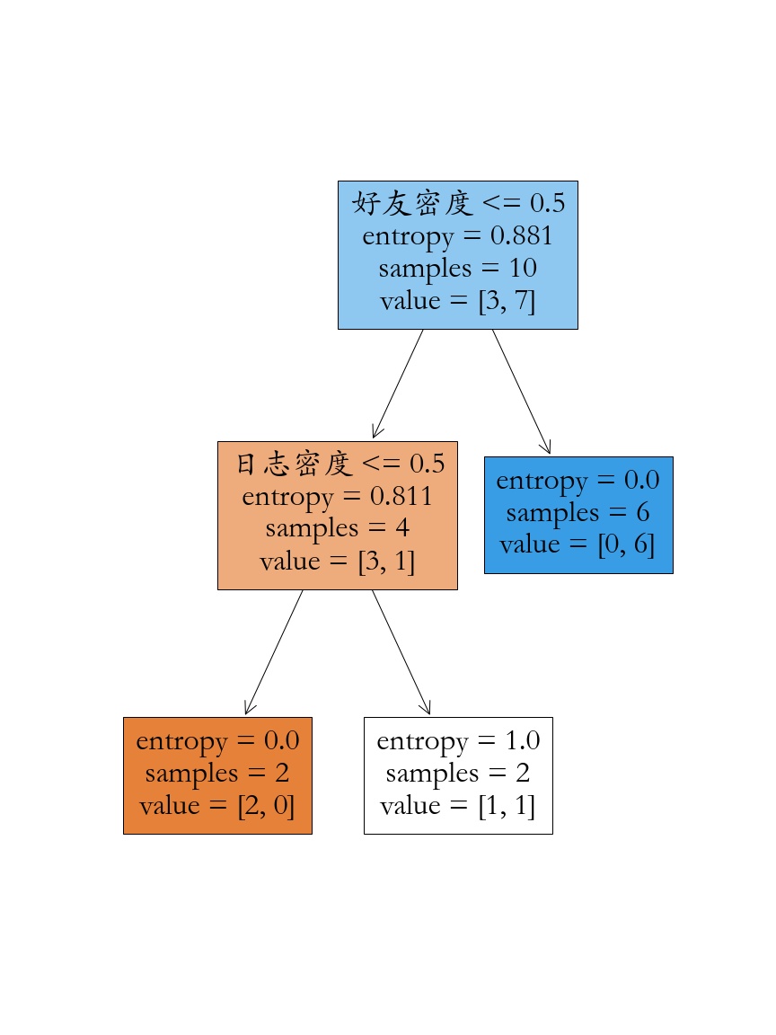

Another Way of Data Visualization, Installation Tutorial

from sklearn.datasets import load_iris
from sklearn.tree import DecisionTreeClassifier
import graphviz
from sklearn import tree
model = DecisionTreeClassifier(criterion='entropy')
model.fit(X,y)
dot_data = tree.export_graphviz(model, out_file=None,
                            feature_names= X.columns,# Feature names
                            class_names=np.unique(y),# Class names
                            filled=True, # Fill color
                            rounded=True) # Rounded corners
graph = graphviz.Source(dot_data)
graph.render('Account',format='png')

Modify Chinese Garbled Characters

import re
# Open dot_data.dot and modify fontname="Supported Chinese font"
f = open('Account', 'r', encoding='utf-8')
with open('./Account2', 'w', encoding="utf-8") as file:
    file.write(re.sub(r'fontname=helvetica', 'fontname=Fangsong', f.read()))
f.close()
# Load from the file and display
graph = graphviz.Source.from_file('./Account2')
graph.render('Account')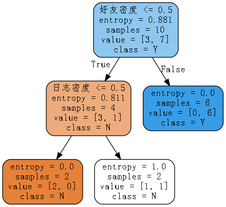

2.3 Information Entropy

• After constructing a tree, the data becomes ordered (before construction, there was a pile of messy data; after constructing a tree, it becomes neatly arranged). What measure should be used to represent whether the data is ordered: information entropy.

• In physics, the second law of thermodynamics (entropy) describes the degree of chaos of a closed system.

  

• Information entropy is similar to the entropy in physics.

  

  $H(x) = -\sum\limits_{i = 1}^n p(x)\log_2p(x)$

• $H(x) = \sum\limits_{i = 1}^n p(x)\log_2\frac{1}{p(x)}$

2.4 Information Gain

Information gain is the degree to which the uncertainty of an event decreases after knowing a certain condition. It is written as g(X,Y). Its calculation method is entropy minus conditional entropy, as follows:

g(X,y) \rm = H(Y) - H(Y|X)

It represents the extent to which the uncertainty of the original event decreases after knowing a certain condition.

2.5 Manually Calculate and Implement Decision Tree Classification

Data Integration

X['Real User'] = y
X

Calculate the Information Entropy Before Partitioning

s = X['Real User']
p = s.value_counts()/s.size
(p * np.log2(1/p)).sum()

Partition According to Log Density

x = X['Log Density'].unique()
x.sort()
# How to partition? Divide it into two parts
for i in range(len(x) - 1):
    split = x[i:i+2].mean()
    cond = X['Log Density'] <= split
    # Probability distribution
    p = cond.value_counts()/cond.size
    # According to the condition partitioning, the probability distribution on both sides
    indexs =p.index
    entropy = 0
    for index in indexs:
        user = X[cond == index]['Real User']
        p_user = user.value_counts()/user.size
        entropy += (p_user * np.log2(1/p_user)).sum() * p[index]
    print(split,entropy)

Screen the Optimal Partition Condition

columns = ['Log Density','Friend Density','Real Avatar']
lower_entropy = 1
condition = {}
for col in columns:
    x = X[col].unique()
    x.sort()
    print(x)
    # How to partition? Divide it into two parts
    for i in range(len(x) - 1):
        split = x[i:i+2].mean()
        cond = X[col] <= split
        # Probability distribution
        p = cond.value_counts()/cond.size
        # According to the condition partitioning, the probability distribution on both sides
        indexs =p.index
        entropy = 0
        for index in indexs:
            user = X[cond == index]['Real User']
            p_user = user.value_counts()/user.size
            entropy += (p_user * np.log2(1/p_user)).sum() * p[index]
        print(col,split,entropy)
        if entropy < lower_entropy:
            condition.clear()
            lower_entropy = entropy
            condition[col] = split
print('The best partitioning condition is:',condition)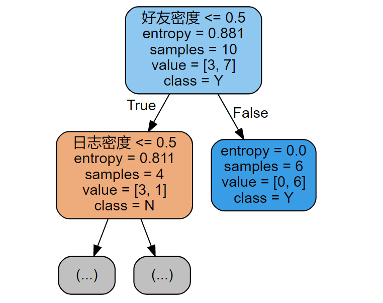

Further Partitioning

cond = X['Friend Density'] < 0.5
X_ = X[cond]
columns = ['Log Density','Real Avatar']
lower_entropy = 1
condition = {}
for col in columns:
    x = X_[col].unique()
    x.sort()
    print(x)
    # How to partition? Divide it into two parts
    for i in range(len(x) - 1):
        split = x[i:i+2].mean()
        cond = X_[col] <= split
        # Probability distribution
        p = cond.value_counts()/cond.size
        # According to the condition partitioning, the probability distribution on both sides
        indexs =p.index
        entropy = 0
        for index in indexs:
            user = X_[cond == index]['Real User']
            p_user = user.value_counts()/user.size
            entropy += (p_user * np.log2(1/p_user)).sum() * p[index]
        print(col,split,entropy)
        if entropy < lower_entropy:
            condition.clear()
            lower_entropy = entropy
            condition[col] = split
print('The best partitioning condition is:',condition)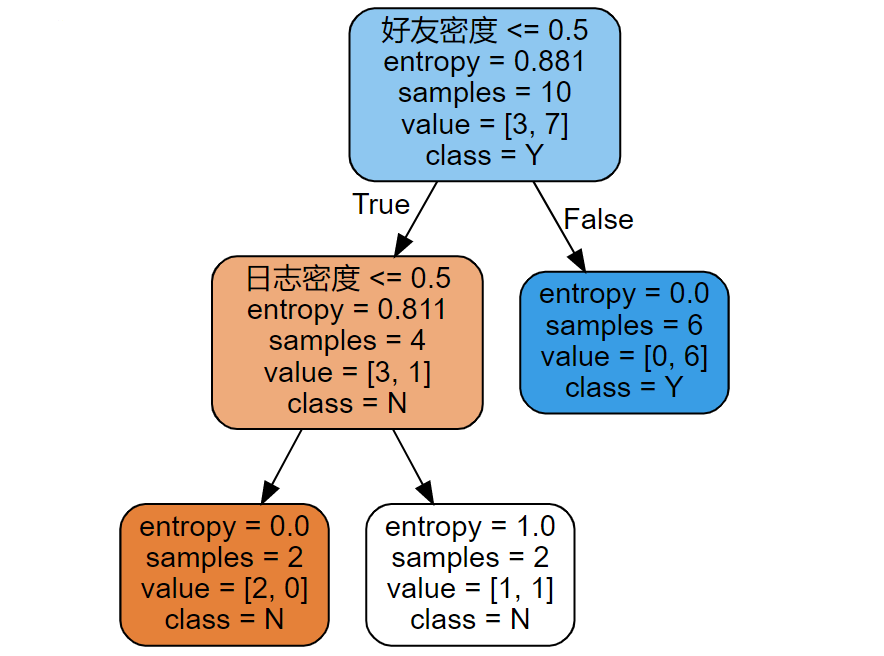

3. Decision Tree Splitting Indicators

Common splitting conditions are:

• Information gain
• Gini coefficient
• Information gain ratio
• MSE (for regression problems)

3.1 Information Entropy (ID3)

In information theory, entropy is called the amount of information, that is, entropy is a measure of uncertainty. From the perspective of cybernetics, it should be called uncertainty. Shannon, the founder of information theory, proposed an information measure based on a probability statistical model in his work A Mathematical Theory of Communication. He defined information as "something used to eliminate uncertainty". In the information world, the higher the entropy, the more information can be transmitted, and the lower the entropy, the less information is transmitted. Let's illustrate with an example. Suppose Dammi has four requirements when buying clothes, namely color, size, style, and design year, while Sara only has requirements for color and size. Then, in terms of buying clothes, Dammi has more choices, so the uncertainty factor is greater. Ultimately, Dammi obtains more information, that is, the entropy is greater. So the amount of information = entropy = uncertainty, which is easy to understand. When describing a decision tree, we use entropy to represent impurity.

The corresponding formula is as follows:

$H(x) = -\sum \limits_{i = 1}^n p(x)\log_2p(x)$

The greater the change in entropy, the purer the partition, and the greater the information gain~

3.2 Gini Coefficient (CART)

The Gini coefficient is a commonly used indicator internationally to measure the income gap among residents in a country or region.

The maximum value of the Gini coefficient is "1", and the minimum value is equal to "0". The closer the Gini coefficient is to 0, the more equal the income distribution is. According to international practice, an income below 0.2 is regarded as absolute income equality, 0.2-0.3 is regarded as relatively equal income; 0.3-0.4 is regarded as relatively reasonable income; 0.4-0.5 is regarded as a relatively large income gap, and when the Gini coefficient reaches above 0.5, it indicates a large income disparity.

The actual value of the Gini coefficient can only be between 0 and 1. The smaller the Gini coefficient, the more average the income distribution is, and the larger the Gini coefficient, the more uneven the income distribution is. Internationally, 0.4 is usually regarded as the warning line of the gap between the rich and the poor, and a value greater than this is likely to lead to social unrest.

The smaller the Gini coefficient, the purer the data in the set. Therefore, we can calculate the value before splitting, partition the dataset according to a certain dimension, and then calculate the Gini coefficients of multiple nodes.

The corresponding formula is as follows:

\rm gini = \sum\limits_{i = 1}^np_i(1 - p_i)

When classifying data, the greater the change in the Gini coefficient, the purer the partition, and the better the effect~

3.3 Information Gain Ratio

In the final mathematics exam of the university, there are only single-choice questions. For a student who has not studied at all, how can he pass the exam?

The probability that each of the 4 options is the correct option is 1/4. Then the entropy of the answers to the single-choice questions is:

H(Y) \rm = -0.25\log_2(0.25) \times 4 = 2bit

There is a secret trick for doing single-choice questions in the circle of top students: choose the shortest one when there are three long options and one short option, and choose the longest one when there are three short options and one long option. Let's assume that the secret trick of top students is generally correct.

If in a certain exam, 10% of the single-choice questions are three long and one short, and 10% of the questions are three short and one long. Calculate the conditional entropy of the single-choice questions in this exam regarding the length of the questions:

Question Type	Probability of Answers	Probability of Questions
Three Long and One Short	(1,0,0,0) Entropy is 0, the result is determined!	10%
Three Short and One Long	(1,0,0,0) Entropy is 0	10%
Same Length	(0.25,0.25,0.25,0.25) Entropy is 2	80%

Calculate the conditional entropy (the condition is: different types of questions)

H(Y|X) \rm = 0.1\times 0 + 0.1 \times 0 + 0.8 \times 2 = 1.6bit

Then the information gain is:

g(X,Y) \rm = H(Y) - H(Y|X) = 2 - 1.6 = 0.4bit

The information gain ratio adds a penalty term on the basis of information gain, and the penalty term is the intrinsic value of the feature.

It is written as gr(X,Y). It is defined as the information gain divided by the intrinsic value of the feature, as follows:

$gr(X,Y) = \frac{g(X,Y)}{Info(X)}$

$Info(X) = -\sum\limits_{v \in values(X)}\frac{num(v)}{num(X)}\log_2{\frac{num(v)}{num(X)}}$

Calculate the information gain ratio of the above case of the length of single-choice questions:

$Info(X) = -(0.1 \times \log_20.1 \times 2 + 0.8 \times \log_20.8) = 0.92$

$gr(X,Y) = \frac{g(X,Y)}{Info(X)} = \frac{0.4}{0.92} = 0.43$

For attributes with more values, especially some continuous numerical values, this single attribute can partition all the samples, making the sample sets under all branches "pure" (in the most extreme case, each leaf node has only one sample). The greater the information gain of an attribute, the stronger the ability of the attribute to reduce the entropy of the samples, and the stronger the ability of this attribute to change the data from uncertainty to certainty. Therefore, for attributes with more values, it is easier to make the data more "pure" (especially for continuous numerical values), and its information gain is greater. The decision tree will first select this attribute as the vertex of the tree. As a result, the trained tree is huge and has a very shallow depth, and such a partition is extremely unreasonable.

C4.5 uses the information gain ratio. On the basis of information gain, it divides by a term of split information to penalize attributes with more values. Thus, the partition becomes more reasonable!

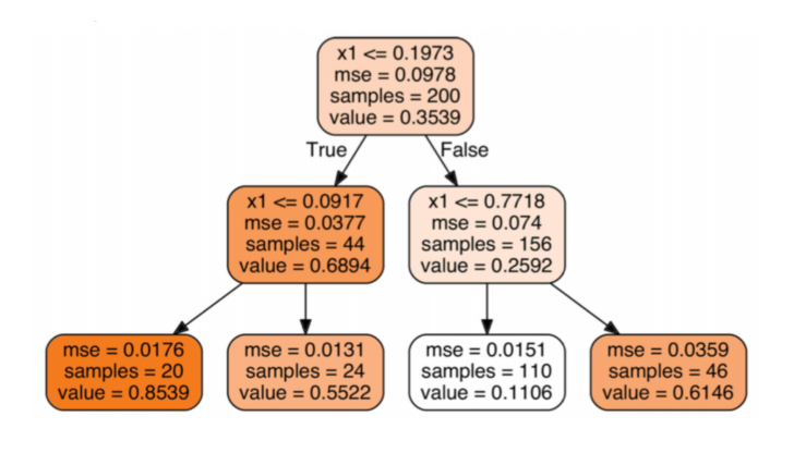
3.4 MSE

It is used for regression trees and will be introduced in detail in the following chapters.

4. Code Practice of Iris Classification

4.1 Decision Tree Classification of the Iris Dataset

import numpy as np
from sklearn.tree import DecisionTreeClassifier
from sklearn import datasets
from sklearn.model_selection import train_test_split
from sklearn import tree
import matplotlib.pyplot as plt

X,y = datasets.load_iris(return_X_y=True)

# Randomly split
X_train,X_test,y_train,y_test = train_test_split(X,y,random_state = 256)

# max_depth adjusts the depth of the tree: pruning operation
# By default, max_depth is the maximum depth, extending until the data is completely partitioned.
model = DecisionTreeClassifier(max_depth=None,criterion='entropy')
model.fit(X_train,y_train)
y_ = model.predict(X_test)
print('The true class is:',y_test)
print('The prediction of the algorithm is:',y_)
print('The accuracy is:',model.score(X_test,y_test))
# The decision tree provides the predict_proba method. It is found that the return value of this method is either 0 or 1.
model.predict_proba(X_test)

4.2 Visualization of the Decision Tree

import graphviz
from sklearn import tree
# Export data
dot_data = tree.export_graphviz(model,feature_names=fn,
                     class_names=iris['target_names'],# Class names
                     filled=True, # Fill color
                     rounded=True,)
graph = graphviz.Source(dot_data)
graph.render('iris')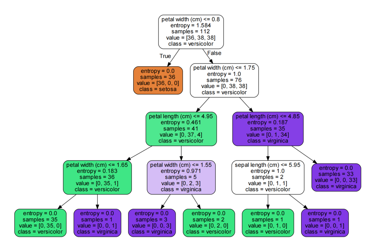

4.3 Pruning of the Decision Tree

# Set the size of the picture
# The iris has 4 attributes
iris = datasets.load_iris()

X = iris['data']
y = iris['target']
fn = iris['feature_names']
# Randomly split
X_train,X_test,y_train,y_test = train_test_split(X,y,random_state = 256)

# max_depth adjusts the depth of the tree: pruning operation
# By default, max_depth is the maximum depth, extending until the data is completely partitioned.
# min_impurity_decrease (minimum impurity for node partitioning) If the impurity (Gini coefficient, information gain, mean squared error) of a certain node is less than this threshold, the node will no longer generate child nodes.
# max_depth (maximum depth of the decision tree); min_samples_split (minimum number of samples required for internal node re-partitioning)
# min_samples_leaf (minimum number of samples in leaf nodes); max_leaf_nodes (maximum number of leaf nodes)
model = DecisionTreeClassifier(criterion='entropy',min_impurity_decrease=0.2)
model.fit(X_train,y_train)
y_ = model.predict(X_test)
print('The true class is:',y_test)
print('The prediction of the algorithm is:',y_)
print('The accuracy is:',model.score(X_test,y_test))
# Export data
dot_data = tree.export_graphviz(model,feature_names=fn,
                     class_names=iris['target_names'],# Class names
                     filled=True, # Fill color
                     rounded=True,)
graph = graphviz.Source(dot_data)
graph.render('./13-iris-pruning')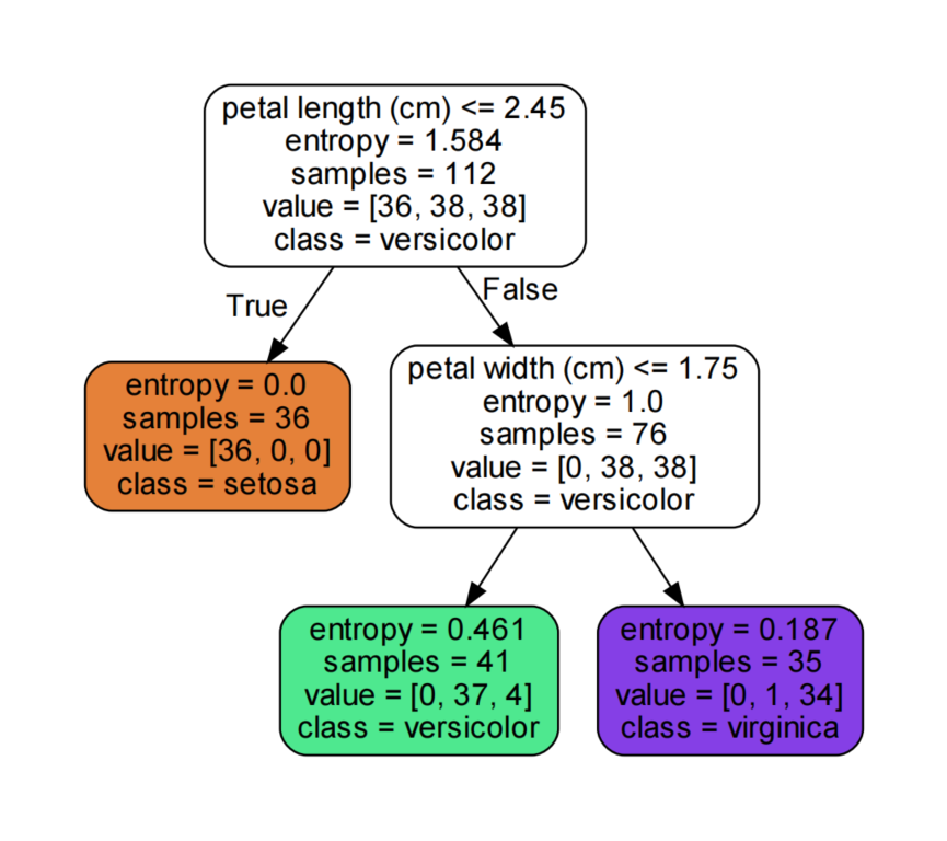

4.4 Selecting Appropriate Hyperparameters and Visualization

import numpy as np
from sklearn.tree import DecisionTreeClassifier
from sklearn import datasets
from sklearn.model_selection import train_test_split
from sklearn import tree
import matplotlib.pyplot as plt

X,y = datasets.load_iris(return_X_y=True)

# Randomly split
X_train,X_test,y_train,y_test = train_test_split(X,y,random_state = 256)
depth = np.arange(1,16)
err = []
for d in depth:
    model = DecisionTreeClassifier(criterion='entropy',max_depth=d)
    model.fit(X_train,y_train)
    score = model.score(X_test,y_test)
    err.append(1 - score)
    print('The error rate is %0.3f%%' % (100 * (1 - score)))
plt.rcParams['font.family'] = 'STKaiti'
plt.plot(depth,err,'ro-')
plt.xlabel('Depth of the Decision Tree',fontsize = 18)
plt.ylabel('Error Rate',fontsize = 18)
plt.title('Selecting the Appropriate Depth of the Decision Tree')
plt.grid()
plt.savefig('./14-selecting-hyperparameters.png',dpi = 200)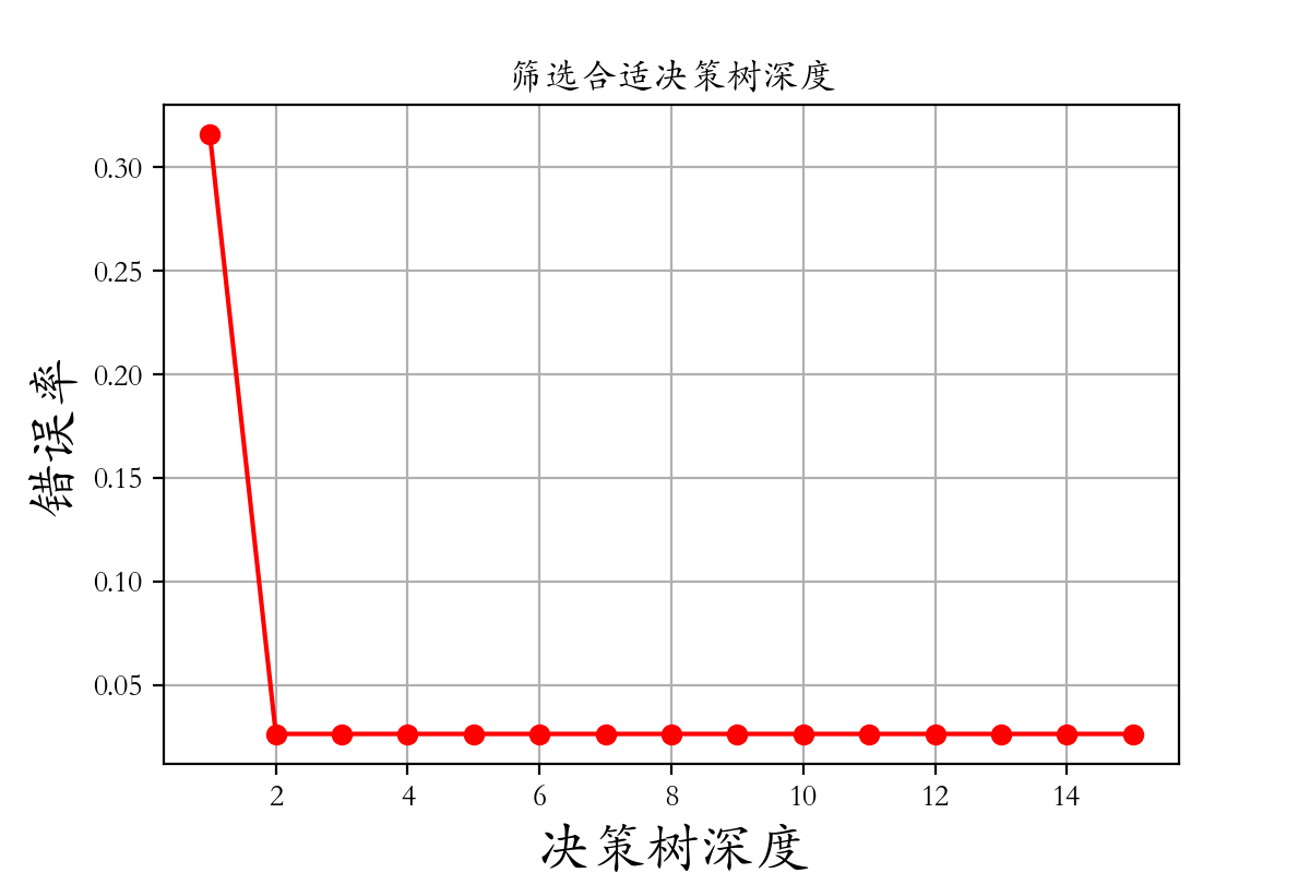

4.5 By-products of the Decision Tree

• Feature Importance

  model.feature_importances_