Logistic Regression for Binary Classification

From Generalized Linear Regression to Logistic Regression

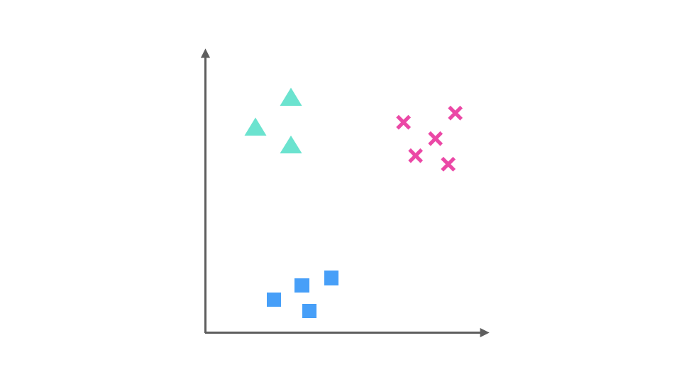
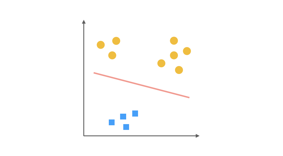
What is Logistic Regression?

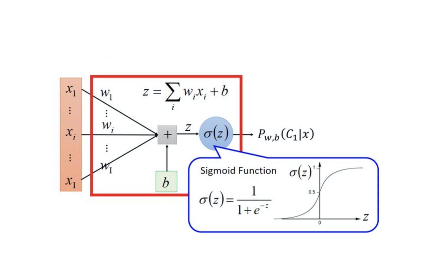
Logistic Regression is not a regression algorithm but a classification algorithm. It is based on Multivariate Linear Regression, making it a linear classifier. A key component of Logistic Regression is the Sigmoid function, which follows an S-shaped curve:

$f(x) = \frac{1}{1 + e^{-x}}$

This function has a useful property where its derivative can be expressed in terms of the function itself:

$f'(x) = \frac{e^{-x}}{(1 + e^{-x})^2} = f(x) \cdot (1 - f(x))$

Here's the Python implementation and plotting code for the Sigmoid function:

import numpy as np
import matplotlib.pyplot as plt

def sigmoid(x):
    return 1 / (1 + np.exp(-x))

x = np.linspace(-5, 5, 100)
y = sigmoid(x)
plt.plot(x, y, color='green')
plt.show()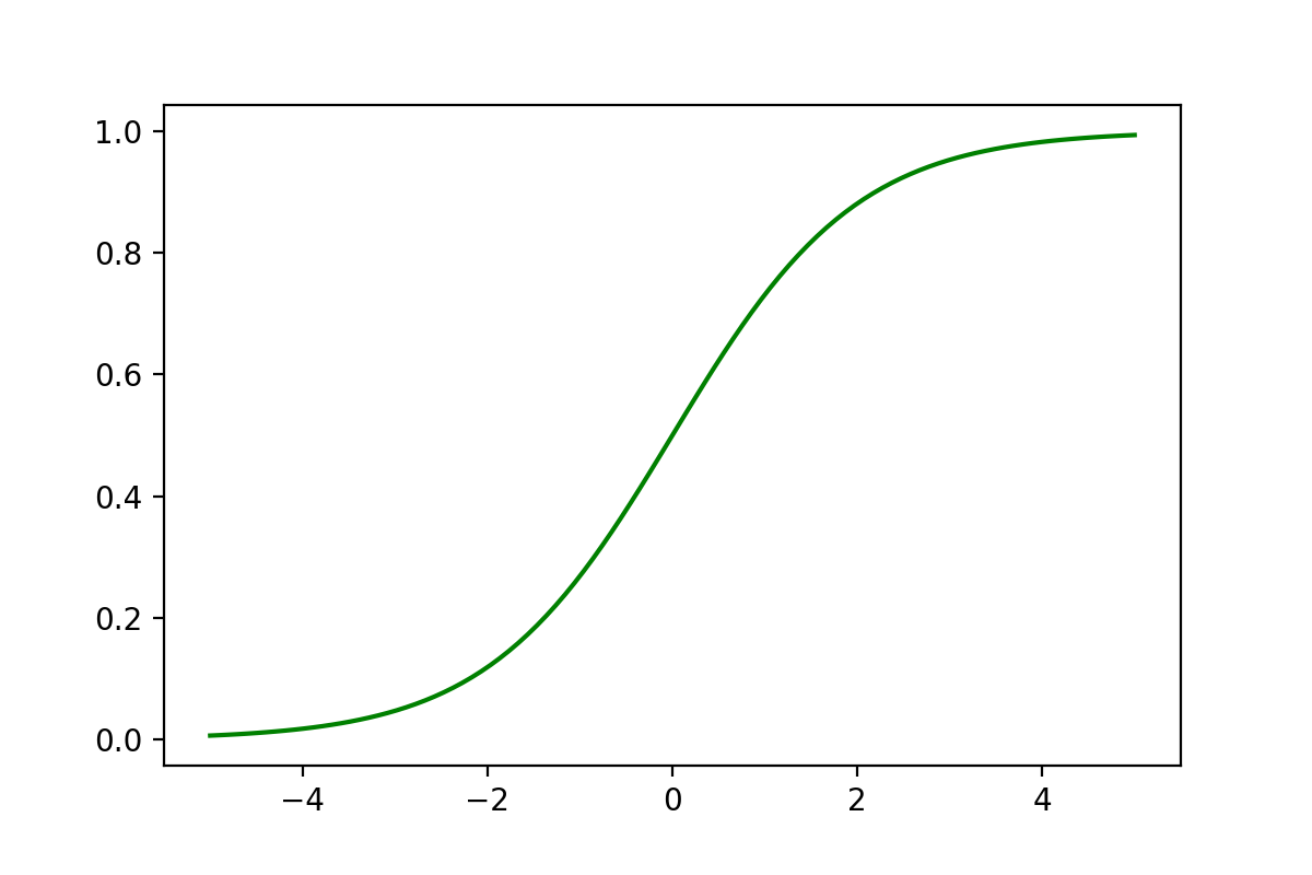

Sigmoid Function Introduction

Logistic Regression scales the results of Multivariate Linear Regression between 0 and 1. Values of $h_{\theta}(x)$ closer to 1 indicate positive examples, while values closer to 0 indicate negative examples. The classification boundary is set at 0.5:

$h_{\theta}(x) = g(\theta^T x) = \frac{1}{1 + e^{-\theta^T x}}$

When $h_{\theta}(x) = 0.5$, which means $\theta^T x = 0$, we find the solution for $\theta$.

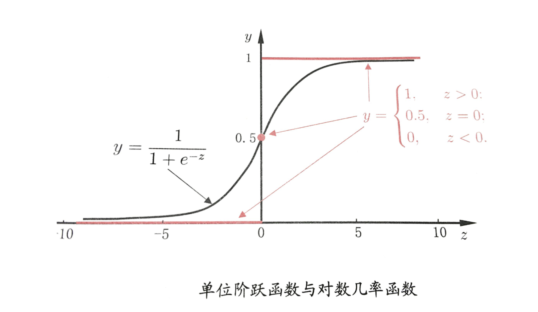
The solution process is as follows:

Bernoulli Distribution for Binary Classification

In binary classification, the probabilities of positive and negative examples sum to 1. The Bernoulli distribution describes trials with two possible outcomes, with the probability function:

$f(x | p) = \begin{cases} p^x (1 - p)^{1 - x}, & x = 1, 0 \\ 0, & x \neq 1, 0 \end{cases}$

In Logistic Regression, positive examples are labeled as 1 and negative examples as 0.

Logistic Regression Formula Derivation

Loss Function Derivation

Logistic Regression uses the Maximum Likelihood Estimation to find the $\theta$ that maximizes the probability of the training data:

$P(y | x; \theta) = \begin{cases} h_{\theta}(x), & y = 1 \\ 1 - h_{\theta}(x), & y = 0 \end{cases}$

This can be combined as:

$P(y | x; \theta) = (h_{\theta}(x))^y (1 - h_{\theta}(x))^{1 - y}$

The likelihood function is:

$L(\theta) = \prod_{i=1}^n (h_{\theta}(x^{(i)}))^{y^{(i)}} (1 - h_{\theta}(x^{(i)}))^{1 - y^{(i)}}$

Taking the natural logarithm gives the log-likelihood function:

$l(\theta) = \sum_{i=1}^n \left[ y^{(i)} \ln(h_{\theta}(x^{(i)})) + (1 - y^{(i)}) \ln(1 - h_{\theta}(x^{(i)})) \right]$

The loss function is:

$J(\theta) = -l(\theta) = -\sum_{i=1}^n \left[ y^{(i)} \ln(h_{\theta}(x^{(i)})) + (1 - y^{(i)}) \ln(1 - h_{\theta}(x^{(i)})) \right]$

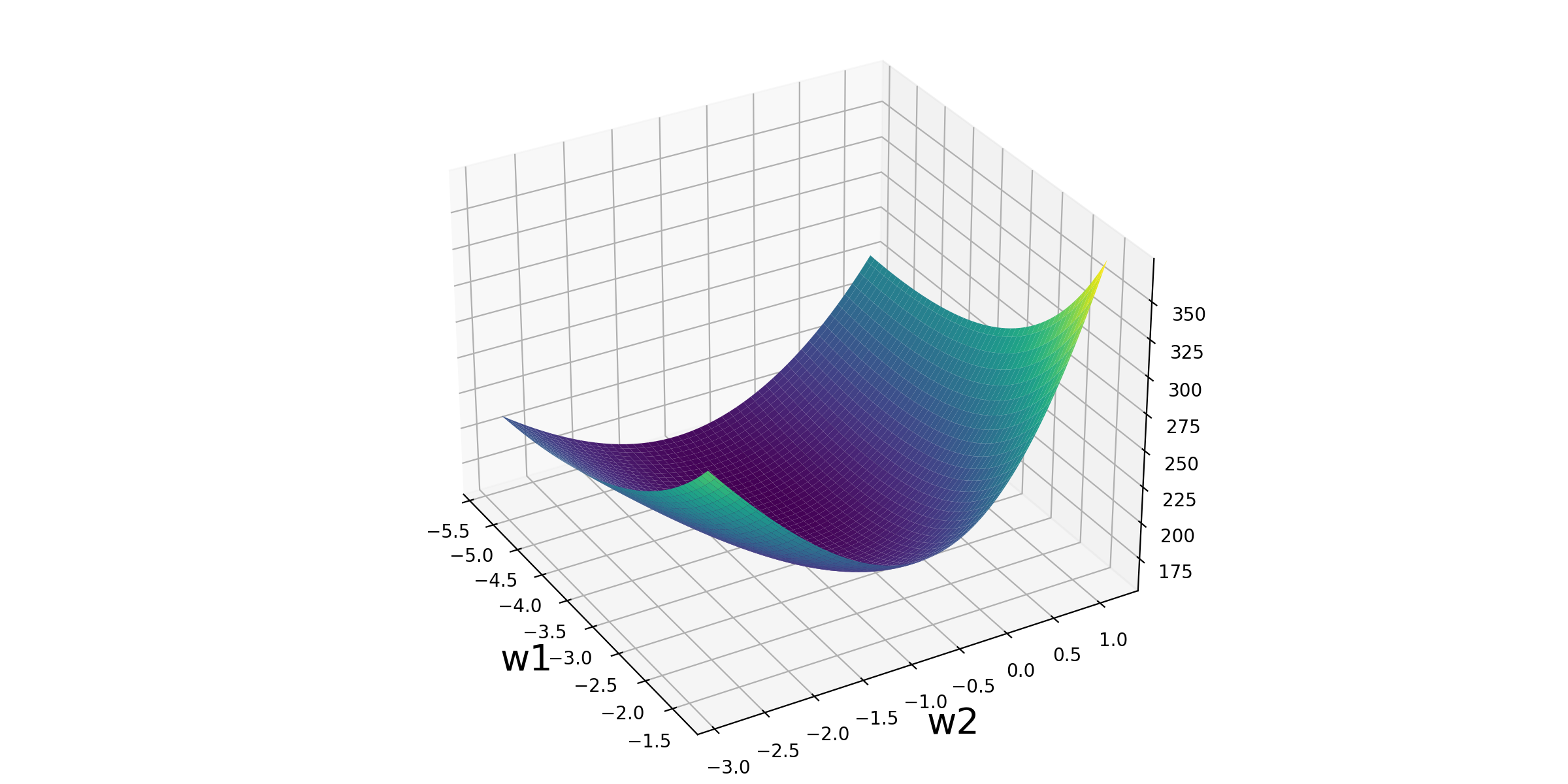
Visualization of the Loss Function

Here's the Python code to visualize the Logistic Regression loss function:

from sklearn import datasets
from sklearn.linear_model import LogisticRegression
import numpy as np
import matplotlib.pyplot as plt
from mpl_toolkits.mplot3d import Axes3D
from sklearn.preprocessing import scale

# Load breast cancer data
data = datasets.load_breast_cancer()
X, y = scale(data['data'][:, :2]), data['target']

# Find optimal solution
lr = LogisticRegression()
lr.fit(X, y)

# Extract parameters
w1 = lr.coef_[0, 0]
w2 = lr.coef_[0, 1]

# Define sigmoid and loss functions
def sigmoid(X, w1, w2):
    z = w1 * X[0] + w2 * X[1]
    return 1 / (1 + np.exp(-z))

def loss_function(X, y, w1, w2):
    loss = 0
    for x_i, y_i in zip(X, y):
        p = sigmoid(x_i, w1, w2)
        loss += -y_i * np.log(p) - (1 - y_i) * np.log(1 - p)
    return loss

# Parameter value space
w1_space = np.linspace(w1 - 2, w1 + 2, 100)
w2_space = np.linspace(w2 - 2, w2 + 2, 100)
loss1_ = np.array([loss_function(X, y, i, w2) for i in w1_space])
loss2_ = np.array([loss_function(X, y, w1, i) for i in w2_space])

# Data visualization
fig1 = plt.figure(figsize=(12, 9))
plt.subplot(2, 2, 1)
plt.plot(w1_space, loss1_)
plt.subplot(2, 2, 2)
plt.plot(w2_space, loss2_)
w1_grid, w2_grid = np.meshgrid(w1_space, w2_space)
loss_grid = loss_function(X, y, w1_grid, w2_grid)
plt.subplot(2, 2, 3)
plt.contour(w1_grid, w2_grid, loss_grid, 20)
plt.subplot(2, 2, 4)
plt.contourf(w1_grid, w2_grid, loss_grid, 20)
plt.savefig('/post/LogisticRegression/4-损失函数可视化.png', dpi=200)

# 3D visualization
fig2 = plt.figure(figsize=(12, 6))
ax = Axes3D(fig2)
ax.plot_surface(w1_grid, w2_grid, loss_grid, cmap='viridis')
plt.xlabel('w1', fontsize=20)
plt.ylabel('w2', fontsize=20)
ax.view_init(30, -30)
plt.savefig('/post/LogisticRegression/5-损失函数可视化.png', dpi=200)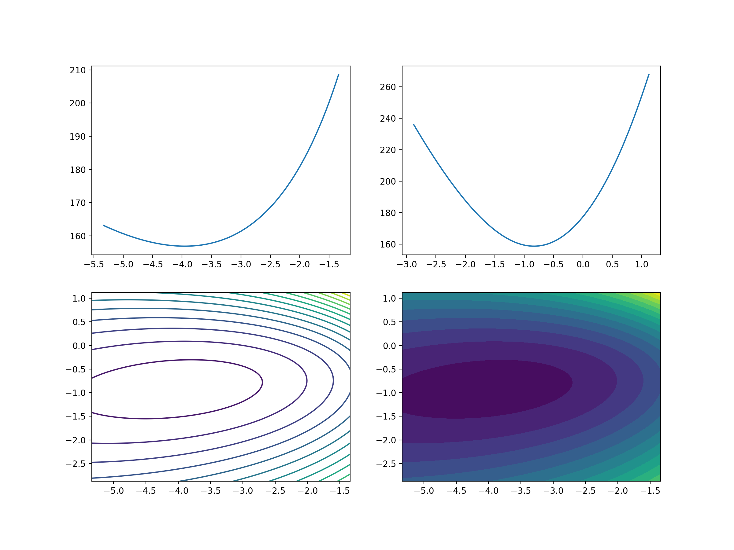

Logistic Regression Update Formula

Function Properties

The parameter update rule for Logistic Regression is similar to that of Linear Regression:

$\theta_j^{t + 1} = \theta_j^t - \alpha \frac{\partial}{\partial \theta_j} J(\theta)$

where $\alpha$ is the learning rate.

The Logistic Regression function and its derivative have the following properties:

$h_{\theta}(x) = g(\theta^T x) = \frac{1}{1 + e^{-z}}$

$g'(z) = g(z) \cdot (1 - g(z))$

Derivative Process

Derivative of the Logistic Regression loss function:

$\frac{\partial}{\partial \theta_j} J(\theta) = \sum_{i=1}^n (h_{\theta}(x^{(i)}) - y^{(i)}) x_j^{(i)}$

Parameter update rule:

$\theta_j^{t+1} = \theta_j^t - \alpha \sum_{i=1}^n (h_{\theta}(x^{(i)}) - y^{(i)}) x_j^{(i)}$

Code Implementation

Here's the implementation of Logistic Regression on the Iris dataset:

import numpy as np
from sklearn import datasets
from sklearn.linear_model import LogisticRegression
from sklearn.model_selection import train_test_split

# Load data
iris = datasets.load_iris()

# Extract and filter data
X = iris['data']
y = iris['target']
cond = y != 2
X = X[cond]
y = y[cond]

# Split data
X_train, X_test, y_train, y_test = train_test_split(X, y)

# Train model
lr = LogisticRegression()
lr.fit(X_train, y_train)

# Make predictions
y_predict = lr.predict(X_test)
print('Actual categories of test data:', y_test)
print('Predicted categories of test data:', y_predict)
print('Prediction probabilities of test data:\n', lr.predict_proba(X_test))

# Linear equation and sigmoid function
b = lr.intercept_
w = lr.coef_

def sigmoid(z):
    return 1 / (1 + np.exp(-z))

z = X_test.dot(w.T) + b
p_1 = sigmoid(z)
p_0 = 1 - p_1
p = np.concatenate([p_0, p_1], axis=1)
print(p)

Logistic Regression for Multi-class Classification

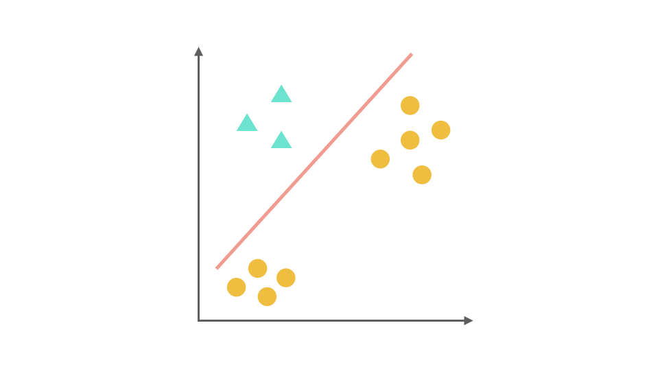
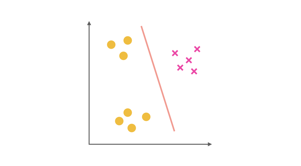
One-Vs-Rest Strategy

For multi-class classification problems, Logistic Regression can be extended using the One-Vs-Rest (OvR) strategy. Taking a three-class problem as an example:

1. Train the first classifier with the first class as positive and the rest as negative.
2. Train the second classifier with the second class as positive and the rest as negative.
3. Train the third classifier with the third class as positive and the rest as negative.

During prediction, calculate the probabilities from each classifier and select the class with the highest probability.

Code Implementation

Here's the implementation of Logistic Regression for the three-class Iris dataset:

import numpy as np
from sklearn import datasets
from sklearn.linear_model import LogisticRegression
from sklearn.model_selection import train_test_split

# Load data
iris = datasets.load_iris()

# Extract data
X = iris['data']
y = iris['target']

# Split data
X_train, X_test, y_train, y_test = train_test_split(X, y)

# Train model using One-Vs-Rest strategy
lr = LogisticRegression(multi_class='ovr')
lr.fit(X_train, y_train)

# Make predictions
y_predict = lr.predict(X_test)
print('Actual categories of test data:', y_test)
print('Predicted categories of test data:', y_predict)
print('Prediction probabilities of test data:\n', lr.predict_proba(X_test))

# Linear equation and sigmoid function
b = lr.intercept_
w = lr.coef_

def sigmoid(z):
    return 1 / (1 + np.exp(-z))

z = X_test.dot(w.T) + b
p = sigmoid(z)
p = p / p.sum(axis=1).reshape(-1, 1)
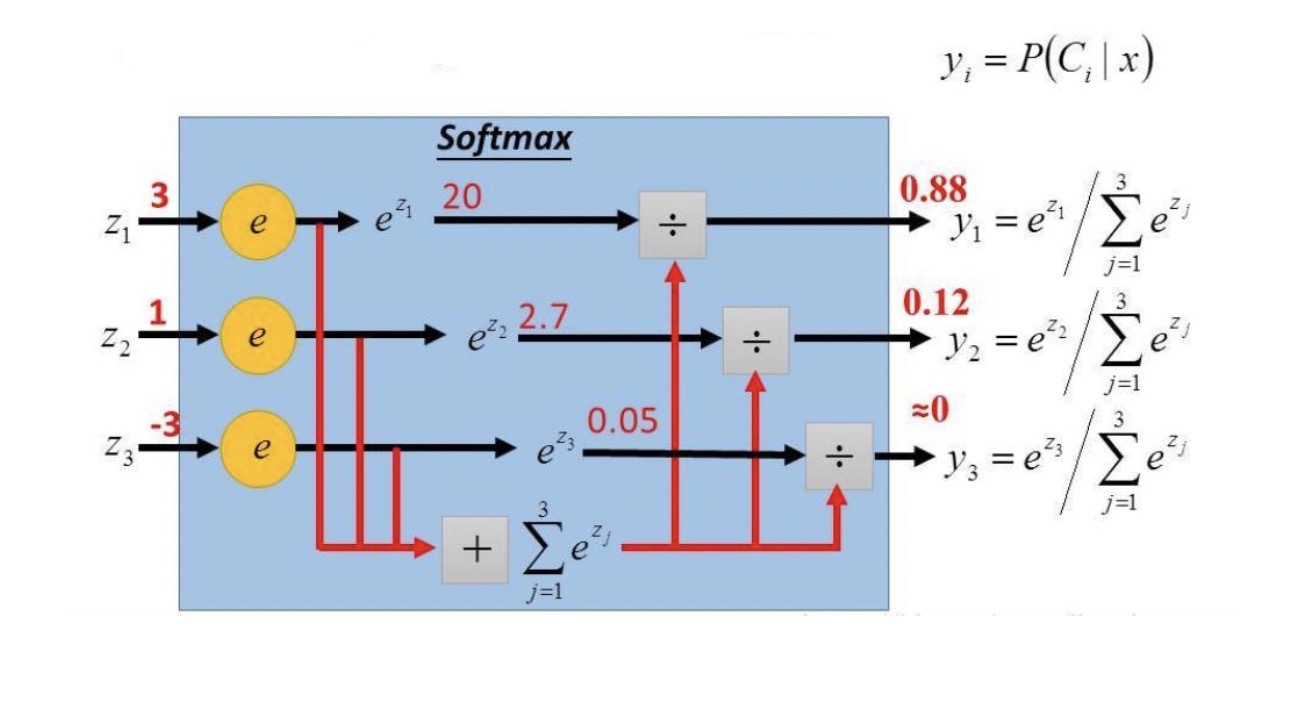
print(p)

Multi-class Softmax Regression

Multinomial Distribution Exponential Family Form

Softmax Regression assumes data follows a multinomial distribution. For a classification problem with k classes, the probability for each class is:

$p(y = i | x; \theta) = \frac{e^{\theta_i^T x}}{\sum_{j=1}^k e^{\theta_j^T x}}$

Generalized Linear Model Derivation of Softmax Regression

The Softmax function converts multiple linear equations' outputs into a probability distribution:

$h_{\theta}(x) = \begin{cases} \frac{e^{\theta_1^T x}}{\sum_{j=1}^k e^{\theta_j^T x}}, & y = 1 \\ \frac{e^{\theta_2^T x}}{\sum_{j=1}^k e^{\theta_j^T x}}, & y = 2 \\ \vdots \\ \frac{e^{\theta_k^T x}}{\sum_{j=1}^k e^{\theta_j^T x}}, & y = k \end{cases}$

Code Implementation

Here's the implementation of Softmax Regression for the three-class Iris dataset:

import numpy as np
from sklearn import datasets
from sklearn.linear_model import LogisticRegression
from sklearn.model_selection import train_test_split

# Load data
iris = datasets.load_iris()

# Extract data
X = iris['data']
y = iris['target']

# Split data
X_train, X_test, y_train, y_test = train_test_split(X, y)

# Train model using Softmax Regression
lr = LogisticRegression(multi_class='multinomial', max_iter=5000)
lr.fit(X_train, y_train)

# Make predictions
y_predict = lr.predict(X_test)
print('Actual categories of test data:', y_test)
print('Predicted categories of test data:', y_predict)
print('Prediction probabilities of test data:\n', lr.predict_proba(X_test))

# Linear equation and softmax function
b = lr.intercept_
w = lr.coef_

def softmax(z):
    return np.exp(z) / np.exp(z).sum(axis=1).reshape(-1, 1)

z = X_test.dot(w.T) + b
p = softmax(z)
print(p)

Comparison of Logistic Regression and Softmax Regression

Logistic Regression as a Special Case of Softmax Regression

When k=2, Softmax Regression simplifies to Logistic Regression:

$h_{\theta}(x) = \frac{1}{1 + e^{\theta^T x}}$

Softmax Loss Function

The loss function for Softmax Regression is the cross-entropy loss:

$J(\theta) = -\sum_{i=1}^n \sum_{j=1}^k I\{y^{(i)} = j\} \log \frac{e^{\theta_j^T x^{(i)}}}{\sum_{l=1}^k e^{\theta_l^T x^{(i)}}}$