Spatial Filtering
Spatial filtering involves moving a spatial template pixel by pixel on the image plane, performing predefined operations between the template and the pixel gray values it covers. The template is also known as a spatial filter, kernel, mask, or window.
Spatial filters are generally used to remove image noise or enhance details, highlighting information of interest while suppressing irrelevant information to improve visual effects for humans or make images more suitable for machine perception or analysis.
Spatial filtering is mainly divided into two categories: smoothing processing and sharpening processing. Smoothing processing is primarily used to handle unimportant details in images and reduce noise. Sharpening processing aims to highlight image details and enhance edges. To achieve satisfactory image enhancement effects, multiple complementary filtering techniques are typically used.
1 Spatial Filtering Fundamentals
The spatial domain refers to the image plane itself, relative to the transform domain. Spatial domain image processing does not involve frequency domain transformation, instead working directly with image pixels. Frequency domain processing transforms the image to the frequency domain for processing, then transforms it back to the spatial domain.
Frequency domain processing mainly includes low-pass filtering and high-pass filtering. Low-pass filtering allows low-frequency signals to pass normally while blocking or attenuating high-frequency signals above a set threshold, useful for noise reduction and equivalent to spatial domain smoothing. High-pass filtering allows high-frequency signals to pass normally while blocking or attenuating low-frequency signals below a set threshold, enhancing edges and contours, and equivalent to spatial domain sharpening.
Filtering in the frequency domain involves passing certain frequency components while rejecting others. Filtering can also be applied in the spatial domain, directly processing images to achieve similar smoothing or sharpening effects as in the frequency domain.
1.1 Mechanism of Spatial Filtering
Spatial filtering works by moving a template across the image pixel by pixel, with each pixel's filter response calculated using a predefined method. If the filter performs linear operations on image pixels, it's called a linear filter; otherwise, it's a nonlinear filter.
Mean filters calculate the average gray value of pixels within the template and are typical linear filters. Statistical ordering filters compare gray values within a given neighborhood, with typical examples being maximum, median, and minimum filters, which are nonlinear.
Mechanism of 3x3 linear spatial filter 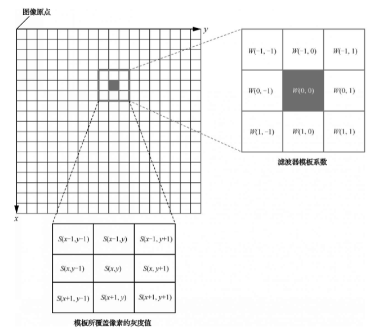
Code for matrix linear spatial filtering:
from skimage import data, color, io
from matplotlib import pyplot as plt
import numpy as np

def corre12d(img, window):
    m = window.shape[0]
    n = window.shape[1]
    # Border extension with 0 gray value filling
    img_border = np.zeros((img.shape[0] + m - 1, img.shape[1] + n - 1))
    img_border[(m - 1) // 2:(img.shape[0] + (m - 1) // 2), (n - 1) // 2:(img.shape[1] + (n - 1) // 2)] = img
    img_result = np.zeros(img.shape)
    for i in range(img_result.shape[0]):
        for j in range(img_result.shape[1]):
            temp = img_border[i:i + m, j:j + n]
            img_result[i, j] = np.sum(np.multiply(temp, window))
    return img_border, img_result

# window is the filter template, img is the original matrix
window = np.array([[1, 0, 0], [0, 0, 0], [0, 0, 2]])
img = np.array([[1, 2, 1, 0, 2, 3], [0, 1, 1, 2, 0, 1],
                [3, 0, 2, 1, 2, 2], [0, 1, 1, 0, 0, 1],
                [1, 1, 3, 2, 2, 0], [0, 0, 1, 0, 1, 0]])

# img_border is the border-extended matrix, img_result is the spatial filtering result
img_border, img_result = corre12d(img, window)
Process of matrix linear spatial filtering 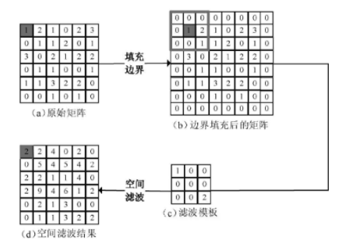
1.2 Spatial Filter Templates
An m×n linear filter template has m×n coefficients that determine its functionality. For a simple 3x3 smoothing filter, coefficients can be set to 1/9.
3x3 linear filter template with coefficients 1/9:
[1/9, 1/9, 1/9]
[1/9, 1/9, 1/9]
[1/9, 1/9, 1/9]
5x5 linear filter template with coefficients 1/9:
[1/25, 1/9, 1/25, 1/9, 1/25]
[1/9, 1/9, 1/9, 1/9, 1/9]
[1/25, 1/9, 1/25, 1/9, 1/25]
[1/9, 1/9, 1/9, 1/9, 1/9]
[1/25, 1/9, 1/25, 1/9, 1/25]
2 Smoothing Processing
Smoothing processing is commonly used for blurring and noise reduction. It replaces pixel gray values with averages or logical operations of neighboring pixels, reducing abrupt gray value changes. However, this can have the negative effect of blurring image edges, which are characterized by abrupt gray value changes.
2.1 Smoothing Linear Spatial Filters
Smoothing linear spatial filters output simple or weighted averages of pixel gray values in a given neighborhood. These are also called mean filters, primarily used for noise reduction and removing unimportant details to make targets easier to detect. The template size should match the details to be removed.
import numpy as np
from scipy import signal
from skimage import data, io
from matplotlib import pyplot as plt


def set_ch():
    from pylab import mpl
    mpl.rcParams['font.sans-serif'] = ['FangSong']
    mpl.rcParams['axes.unicode_minus'] = False


# Define 2D grayscale image spatial filtering function
def correl2d(img, window):
    """
    Implement image spatial correlation using filter
    mode='same' means output size equals input size
    boundary='fill' means fill image edges with constant value before filtering, default is 0

    :param img:
    :param window:
    :return:
    """
    s = signal.correlate2d(img, window, mode='same', boundary='fill')
    return s.astype(np.uint8)


set_ch()
img = data.camera()
# 3x3 box filter template
window1 = np.ones((3, 3)) / (3 ** 2)
# 5x5 box filter template
window2 = np.ones((5, 5)) / (5 ** 2)
# 9x9 box filter template
window3 = np.ones((9, 9)) / (9 ** 2)

# Generate filtering results
img1 = correl2d(img, window1)
img2 = correl2d(img, window2)
img3 = correl2d(img, window3)

plt.figure()
plt.subplot(221)
plt.axis('off')
plt.title('Original Image')
plt.imshow(img, cmap='gray')

plt.subplot(222)
plt.axis('off')
plt.title('3x3')
plt.imshow(img1, cmap='gray')

plt.subplot(223)
plt.axis('off')
plt.title('5x5')
plt.imshow(img2, cmap='gray')

plt.subplot(224)
plt.axis('off')
plt.title('9x9')
plt.imshow(img3, cmap='gray')
plt.show()
Box filter results show smoother water ripples compared to the original image, with distant scenery and the photographer also appearing more blurred. 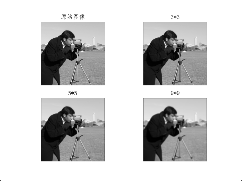
Gaussian smoothing is a widely used spatial filtering method.
import numpy as np
from scipy import signal
from skimage import data, io
from matplotlib import pyplot as plt
import math

def set_ch():
    from pylab import mpl
    mpl.rcParams['font.sans-serif'] = ['FangSong']
    mpl.rcParams['axes.unicode_minus'] = False

# Define 2D grayscale image spatial filtering function
def correl2d(img, window):
    """
    Implement image spatial correlation using filter
    mode='same' means output size equals input size
    boundary='fill' means fill image edges with constant value before filtering, default is 0

    :param img:
    :param window:
    :return:
    """
    s = signal.correlate2d(img, window, mode='same', boundary='fill')
    return s.astype(np.uint8)

# Define 2D Gaussian function
def gauss(i, j, sigma):
    return 1 / (2 * math.pi * sigma ** 2) * math.exp(-(i ** 2 + j ** 2) / (2 * sigma ** 2))

# Define radius x radius Gaussian smoothing template
def gauss_window(radius, sigma):
    window = np.zeros((radius * 2 + 1, radius * 2 + 1))
    for i in range(-radius, radius + 1):
        for j in range(-radius, radius + 1):
            window[i + radius][j + radius] = gauss(i, j, sigma)
    return window / np.sum(window)

set_ch()
img = data.camera()
# 3x3 Gaussian smoothing filter template
window1 = gauss_window(3, 1.0)

# 5x5 Gaussian smoothing filter template
window2 = gauss_window(5, 1.0)

# 9x9 Gaussian smoothing filter template
window3 = gauss_window(9, 1.0)

# Generate filtering results
img1 = correl2d(img, window1)
img2 = correl2d(img, window2)
img3 = correl2d(img, window3)

plt.figure()
plt.subplot(221)
plt.axis('off')
plt.title('Original Image')
plt.imshow(img, cmap='gray')

plt.subplot(222)
plt.axis('off')
plt.title('3x3')
plt.imshow(img1, cmap='gray')

plt.subplot(223)
plt.axis('off')
plt.title('5x5')
plt.imshow(img2, cmap='gray')

plt.subplot(224)
plt.axis('off')
plt.title('9x9')
plt.imshow(img3, cmap='gray')
plt.show()
With the same template size, Gaussian filtering produces less smoothing. Gaussian filtering weights neighboring pixels, giving higher weights to pixels closer to the center. Compared to box filtering, Gaussian filtering produces softer smoothing with better preservation of target details. 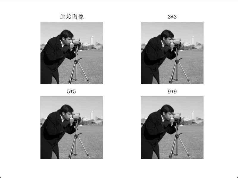
2.2 Statistical Ordering Filters
Statistical ordering filters are typical nonlinear smoothing filters. They sort gray values within the template coverage and select representative values as the filter response. Common types include maximum, median, and minimum filters.
Maximum filters replace pixel values with the maximum in their neighborhood, useful for finding bright spots. Median filters replace values with the median, effective for noise reduction. Minimum filters use the minimum value, helpful for finding dark spots.
Median filters perform well on certain random noise types, producing less blurring than same-sized mean filters. They're particularly effective for impulse noise removal, as they take the median value, eliminating outliers in the neighborhood. This makes images more uniform, reducing isolated bright or dark points.
To observe median filtering's denoising effect, we add impulse noise to an astronaut image and apply a 3x3 median filter.
from scipy import ndimage
from skimage import util, data
from matplotlib import pyplot as plt

img = data.astronaut()[:, :, 0]
# Add impulse noise to image
noise_img = util.random_noise(img, mode='s&p', seed=None, clip=True)
# Median filtering
n = 3
new_img = ndimage.median_filter(noise_img, (n, n))

plt.figure()
plt.axis('off')
plt.imshow(img, cmap='gray')  # Show original image

plt.figure()
plt.axis('off')
plt.imshow(noise_img, cmap='gray')  # Show noisy image

plt.figure()
plt.axis('off')
plt.imshow(new_img, cmap='gray')  # Show denoised image

plt.show()
Original image 
Noisy image 
Denoised image 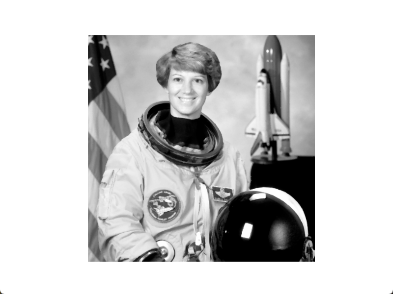
For RGB image spatial filtering, each of the three channels is processed separately.
from scipy import ndimage
from skimage import util, data
from matplotlib import pyplot as plt
import numpy as np

img = data.astronaut()

noise_img = np.zeros(img.shape)
new_img = np.zeros(img.shape)
for i in range(3):
    gray_img = img[:, :, i]
    # Add impulse noise to image
    noise_img[:, :, i] = util.random_noise(gray_img, mode='s&p', seed=None, clip=True)
    # Median filtering
    n = 3
    new_img[:, :, i] = ndimage.median_filter(noise_img[:, :, i], (n, n))

plt.figure()
plt.axis('off')
plt.imshow(img, cmap='gray')  # Show original image

plt.figure()
plt.axis('off')
plt.imshow(noise_img, cmap='gray')  # Show noisy image

plt.figure()
plt.axis('off')
plt.imshow(new_img, cmap='gray')  # Show denoised image

plt.show()
Original image 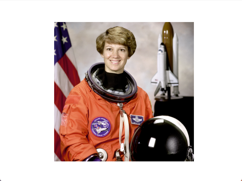
Noisy image 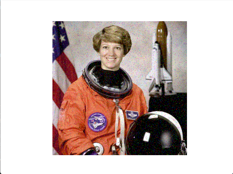
Denoised image 
Maximum filtering is effective for finding image bright spots and reducing pepper noise. Minimum filtering helps find dark spots and reduce salt noise.
from scipy import ndimage
from skimage import util, data
from matplotlib import pyplot as plt
import numpy as np

img = data.astronaut()[:, :, 0]

# Add pepper noise to image
pepper_img = util.random_noise(img, mode='pepper', seed=None, clip=True)
# Add salt noise to image
salt_img = util.random_noise(img, mode='salt', seed=None, clip=True)
n = 3
# Maximum filtering
max_img = ndimage.maximum_filter(pepper_img, (n, n))
# Minimum filtering
min_img = ndimage.minimum_filter(salt_img, (n, n))

plt.figure()
plt.axis('off')
plt.imshow(img, cmap='gray')  # Show original image

plt.figure()
plt.axis('off')
plt.imshow(pepper_img, cmap='gray')  # Show pepper noise image

plt.figure()
plt.axis('off')
plt.imshow(salt_img, cmap='gray')  # Show salt noise image

plt.figure()
plt.axis('off')
plt.imshow(max_img, cmap='gray')  # Show maximum filtered image

plt.figure()
plt.axis('off')
plt.imshow(min_img, cmap='gray')  # Show minimum filtered image

plt.show()
Pepper noise image 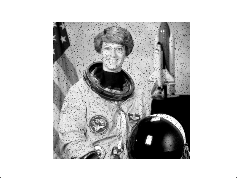
Salt noise image 
Maximum filtered image 
Minimum filtered image 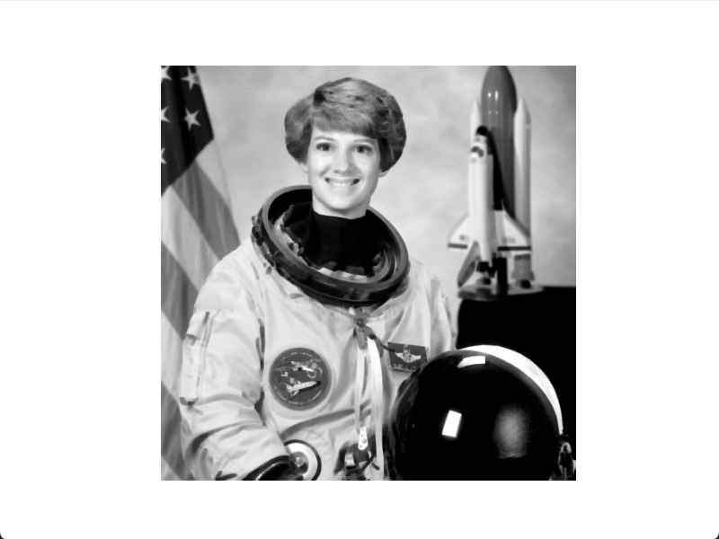
3 Sharpening Processing
Sharpening processing enhances details, edges, contours, and other gray value changes in images while reducing gradual gray value variations. Since differentiation describes the local change rate of a function, image sharpening algorithms are often based on spatial differentiation. Smoothing processing can blur edges and details, so sharpening can be achieved by subtracting smoothed images from original images, known as unsharp masking.
3.1 First-Order Differential Operators
Any first-order differential definition must satisfy: ① Zero differential value in constant gray value areas; ② Non-zero values in changing areas. For discrete cases, differentiation is approximated by differencing.
According to Roberts' criteria, edge detectors should produce clear edges, minimize background noise, and match human perception of edge strength. Code for Roberts edge and gradient images:
from skimage import data, filters
from matplotlib import pyplot as plt

img = data.camera()
# Roberts cross-gradient operator
img_robert_pos = filters.roberts_pos_diag(img)
img_robert_neg = filters.roberts_neg_diag(img)
img_robert = filters.roberts(img)

# Show original image
plt.figure()
plt.imshow(img, cmap='gray')
plt.show()

# Show Roberts positive diagonal edge image
plt.figure()
plt.imshow(img, cmap='gray')
plt.show()

# Show Roberts negative diagonal edge image
plt.figure()
plt.imshow(img, cmap='gray')
plt.show()

# Show Roberts gradient image
plt.figure()
plt.imshow(img, cmap='gray')
plt.show()
Original image 
Roberts positive diagonal edge image 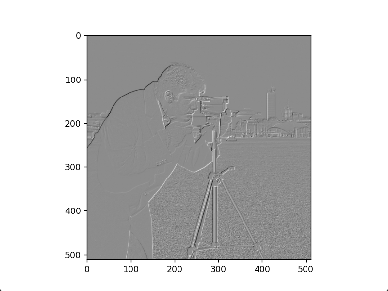
Roberts negative diagonal edge image 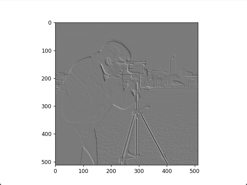
Roberts gradient image 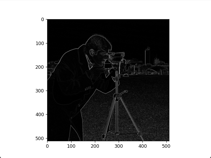
Code for Sobel edge and gradient images:
from skimage import data, filters
from matplotlib import pyplot as plt

img = data.camera()
# Sobel operator
img_sobel_h = filters.sobel_h(img)
img_sobel_v = filters.sobel_v(img)
img_sobel = filters.sobel(img)

# Show original image
plt.figure()
plt.imshow(img, cmap='gray')
plt.show()

# Show horizontal Sobel edge image
plt.figure()
plt.imshow(img_sobel_h, cmap='gray')
plt.show()

# Show vertical Sobel edge image
plt.figure()
plt.imshow(img_sobel_v, cmap='gray')
plt.show()

# Show Sobel gradient image
plt.figure()
plt.imshow(img_sobel, cmap='gray')
plt.show()
Horizontal Sobel edge image 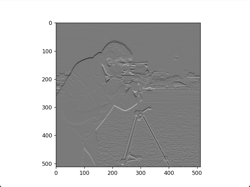
Vertical Sobel edge image 
Sobel gradient image 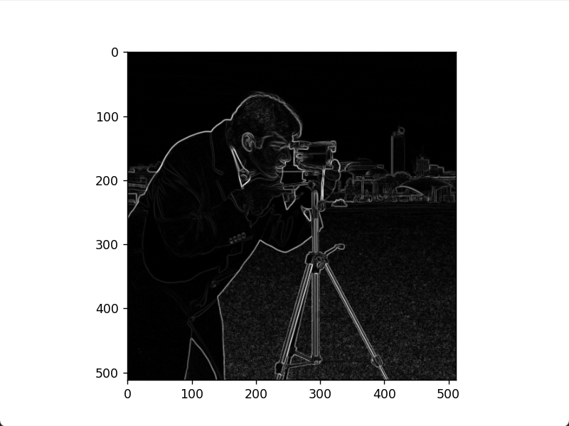
3.2 Second-Order Differential Operators
Any second-order differential definition must satisfy: Zero value in constant gray value areas; non-zero at edges or ramps; zero along ramps.
Applying the Laplacian operator to an image produces a Laplacian image. Adding this to the original image, with a coefficient matching the Laplacian template's center sign, enhances image details. Code:
from skimage import data, filters
from matplotlib import pyplot as plt

img = data.camera()
# Laplacian
img_laplace = filters.laplace(img, ksize=3, mask=None)
img_enhance = img + img_laplace

# Show original image
plt.figure()
plt.imshow(img, cmap='gray')
plt.show()

# Show Laplacian image
plt.figure()
plt.imshow(img_laplace, cmap='gray')
plt.show()

# Show enhanced image
plt.figure()
plt.imshow(img_enhance, cmap='gray')
plt.show()
Original image 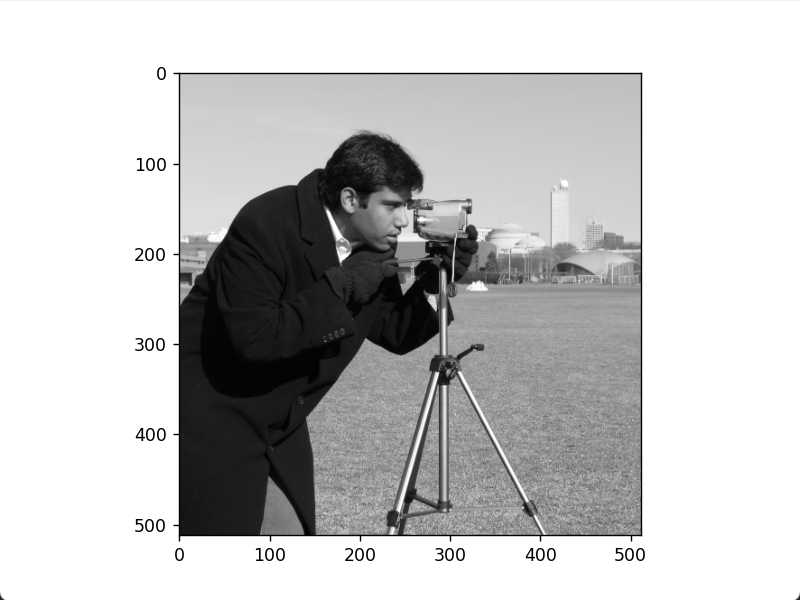
Laplacian image 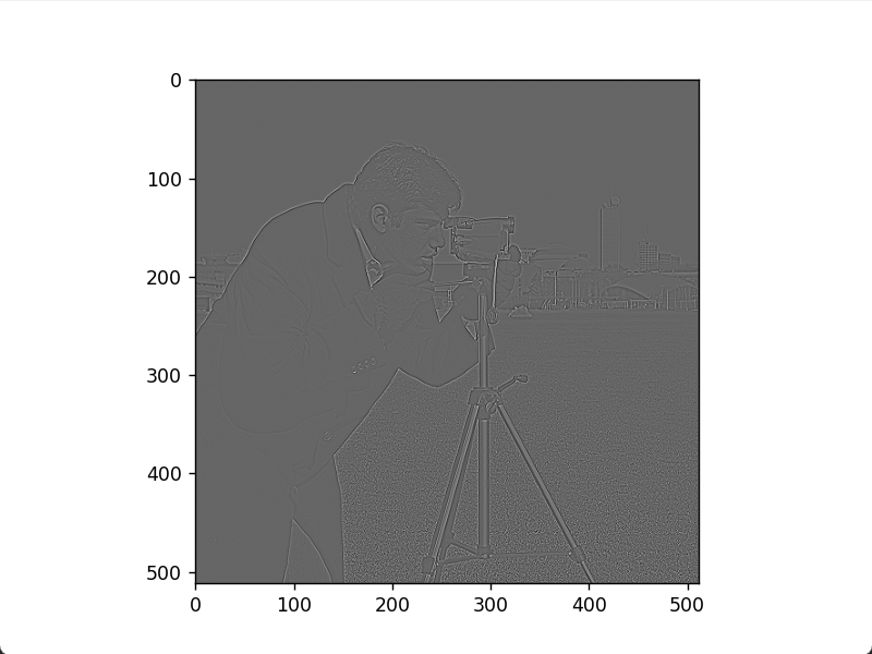
Enhanced image 
First-order differentiation highlights edges more, while second-order is more sensitive to intense gray value changes, emphasizing texture.
3.3 Unsharp Masking
Smoothing can blur edges and details, so sharpening is achieved by subtracting smoothed images from original images. This involves three steps: smoothing to get a blurred image, subtracting to get a difference image, then adding this back to the original.
from skimage import data, filters
from matplotlib import pyplot as plt
from scipy import signal
import numpy as np

def correlate2d(img, window):
    s = signal.correlate2d(img, window, mode='same', boundary='fill')
    return s


img = data.camera()
# 3x3 box filter template
window = np.ones((3, 3)) / (3 ** 2)
img_blur = correlate2d(img, window)
img_edge = img - img_blur
img_enhance = img + img_edge

# Show original image
plt.figure()
plt.imshow(img, cmap='gray')
plt.show()

# Show blurred image
plt.figure()
plt.imshow(img_blur, cmap='gray')
plt.show()

# Show difference image
plt.figure()
plt.imshow(img_edge, cmap='gray')
plt.show()

# Show enhanced image
plt.figure()
plt.imshow(img_enhance, cmap='gray')
plt.show()
Blurred image 
Difference image 
Enhanced image 
4 Hybrid Spatial Enhancement
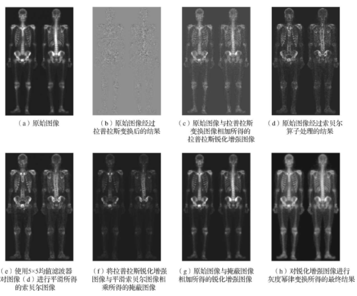
Hybrid spatial enhancement combines smoothing filters, sharpening filters, and gray level stretching for better visual effects. For full-body bone scans with narrow gray ranges and significant noise, single filters are insufficient.
The process involves: Laplacian sharpening for small details, Sobel gradient processing for edges, smoothing gradients for masking, and power-law transformation for dynamic range enhancement. Full-body bone scan enhancement flow: 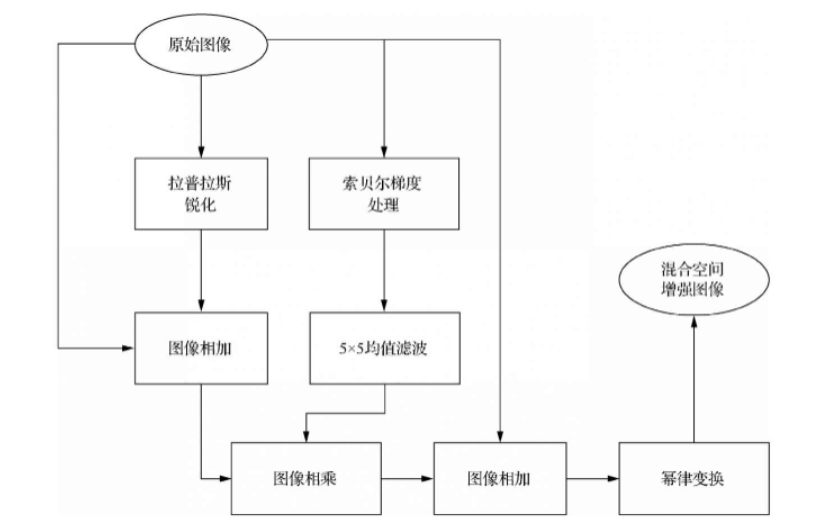
Process description: 1. Laplacian sharpening; 2. Add to original for enhancement; 3. Sobel edge detection; 4. Smooth with 5x5 mean filter; 5. Multiply sharpened image with smoothed gradient; 6. Add masked image to original; 7. Power-law transformation for final result.
from skimage import data, filters, io
from matplotlib import pyplot as plt
import numpy as np

# Image spatial filtering function
def correlate2d(img, window):
    m = window.shape[0]
    n = window.shape[1]
    # Border extension with 0 gray value filling
    img1 = np.zeros((img.shape[0] + m - 1, img.shape[1] + n - 1))
    img1[(m - 1) // 2:(img.shape[0] + (m - 1) // 2), (n - 1) // 2:(img.shape[1] + (n - 1) // 2)] = img
    img2 = np.zeros(img.shape)
    for i in range(img2.shape[0]):
        for j in range(img2.shape[1]):
            temp = img1[i:i + m, j:j + n]
            img2[i, j] = np.sum(np.multiply(temp, window))
    return img2


img = io.imread('boneScan.jpg', as_gray=True)
# img_laplace is the result of Laplacian transform on the original image
window = np.array([[-1, -1, -1], [-1, 8, -1], [-1, -1, -1]])
img_laplace = correlate2d(img, window)
img_laplace = 255 * (img_laplace - img_laplace.min()) / (img_laplace.max() - img_laplace.min())
# Add img and img_laplace to get sharpened image
img_laplace_enhance = img + img_laplace
# img_sobel is the result of Sobel processing on the original image
img_sobel = filters.sobel(img)
# Smooth Sobel image with 5x5 mean filter
window_mean = np.ones((5, 5)) / (5 ** 2)
img_sobel_mean = correlate2d(img_sobel, window_mean)
# Multiply img_laplace_enhance with img_sobel_mean to get masked image
img_mask = img_laplace_enhance * img_sobel_mean
# Add original image with masked image to get final enhanced image
img_sharp_enhance = img + img_mask
# Power-law transformation on img_sharp_enhance for final result
img_enhance = img_sharp_enhance ** 0.5

# Display images
imgList = [img, img_laplace, img_laplace_enhance, img_sobel, img_sobel_mean, img_mask, img_sharp_enhance, img_enhance]
for grayImg in imgList:
    plt.figure()
    plt.axis('off')
    plt.imshow(grayImg, cmap='gray')
    plt.show()