Frequency Filtering

• In his work "Théorie analytique de la chaleur" (The Analytical Theory of Heat), French mathematician Joseph Fourier demonstrated that any periodic function can be decomposed into a series of sine or cosine functions with different frequencies, known as a Fourier series. This method fundamentally transforms spatial information into frequency domain information, allowing spatial domain signal processing problems to be converted into frequency domain signal processing problems.
• Fourier transform can decompose any periodic function into signal components of different frequencies.
• Frequency domain transformation provides a different approach to signal processing. Sometimes problems that are difficult to handle in the spatial domain can be easily addressed through frequency domain transformation.
• To more effectively process digital images, it is often necessary to transform the original image into another space using a specific method, utilize the unique properties of the image in that transformed space to process the image information, and then transform it back to the image space to achieve the desired effect.
• Image transformation is bidirectional. Generally, transforming from the image space to another space is called the forward transform, while transforming from another space back to the image space is called the inverse transform.
• Fourier transform treats images as two-dimensional signals, with the horizontal and vertical directions serving as the coordinate axes of the two-dimensional space, and the domain where the image itself resides is called the spatial domain.
• The rhythm of gray value changes in an image with spatial coordinates can be measured by frequency, referred to as spatial frequency or frequency domain.
• Frequency filtering for digital images involves transforming the original image to the frequency domain through Fourier transform, then processing the image in the frequency domain, and finally transforming it back to the spatial domain using the inverse Fourier transform to obtain the processed image.
• Compared to spatial domain image processing, frequency domain image processing has the following advantages: ① Frequency domain image processing can accomplish tasks that are difficult to achieve in the spatial domain by utilizing the special properties of frequency domain components. ② Frequency domain image processing is more beneficial for explaining image processing, allowing for more intuitive explanations of certain effects produced during the filtering process. ③ Frequency domain filters can serve as a guide for designing spatial domain filters. Frequency domain filters can be converted to spatial domain operations through inverse Fourier transform, allowing for preliminary design in the frequency domain and implementation in the spatial domain.

1 Fourier Transform

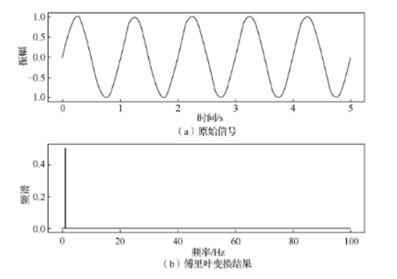
• Fourier transform is a common orthogonal mathematical transformation that decomposes one-dimensional signals or functions into combinations of sine or cosine signals with different frequencies and amplitudes.
• The core contribution of Fourier transform lies in determining the proportion or frequency of each sine or cosine wave, allowing the original signal to be reconstructed from these waves.
• A simple example of Fourier transform:

from matplotlib import pyplot as plt
import numpy as np

# Function to enable Chinese font display
def set_ch():
    from pylab import mpl
    mpl.rcParams['font.sans-serif'] = ['FangSong']
    mpl.rcParams['axes.unicode_minus'] = False

set_ch()

def show(ori_func, sampling_period=5):
    n = len(ori_func)
    interval = sampling_period / n
    # Plot original function
    plt.subplot(2, 1, 1)
    plt.plot(np.arange(0, sampling_period, interval), ori_func, 'black')
    plt.xlabel('Time'), plt.ylabel('Amplitude')
    plt.title('Original Signal')
    # Plot transformed function
    plt.subplot(2, 1, 2)
    frequency = np.arange(n / 2) / (n * interval)
    nfft = abs(ft[range(int(n / 2))] / n)
    plt.plot(frequency, nfft, 'red')
    plt.xlabel('Frequency (Hz)'), plt.ylabel('Spectrum')
    plt.title('Fourier Transform')
    plt.show()

# Generate a sine wave with frequency 1 and angular velocity 2*pi
time = np.arange(0, 5, .005)
x = np.sin(2 * np.pi * 1 * time)
y = np.fft.fft(x)
show(x, y)

• The Fourier transform result of a single sine wave

1.2 Two-dimensional Fourier Transform

• The two-dimensional Fourier transform is essentially a simple extension of the one-dimensional case to two dimensions.
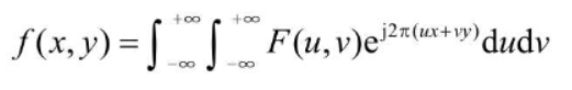
• The inverse transform of the two-dimensional Fourier transform can be represented as:

from matplotlib import pyplot as plt
import numpy as np
from skimage import data

# Function to enable Chinese font display
def set_ch():
    from pylab import mpl
    mpl.rcParams['font.sans-serif'] = ['FangSong']
    mpl.rcParams['axes.unicode_minus'] = False

set_ch()
img = data.camera()
#img = data.checkerboard()
# Perform fast Fourier transform to obtain frequency distribution
f = np.fft.fft2(img)
# By default, the center point is in the upper left corner; shift it to the center
fshift = np.fft.fftshift(f)
# The result of FFT is a complex number; take the absolute value for amplitude
fimg = np.log(np.abs(fshift))
# Display results
plt.subplot(1, 2, 1), plt.imshow(img, 'gray'), plt.title('Original Image')
plt.subplot(1, 2, 2), plt.imshow(fimg, 'gray'), plt.title('Fourier Spectrum')
plt.show()

• The Fourier transform of a checkerboard image
• After Fourier transform, the DC component is proportional to the image mean, while high-frequency components indicate the strength and direction of edges in the image.

2 Properties of Fourier Transform

2.1 Basic Properties of Fourier Transform

① Linearity: If f1(t)↔F1(Ω) and f2(t)↔F2(Ω), then af1(t)+bf2(t)↔aF1(Ω)+bF2(Ω), where a and b are constants. This allows complex signals to be decomposed into simpler components. ② Time-shift: A time shift in the signal results in a linear phase shift in the frequency domain without changing the amplitude. ③ Frequency-shift: Multiplying a signal by a complex exponential in the time domain shifts its spectrum by Ω0 in the frequency domain. ④ Scaling: Compression in the time domain results in expansion in the frequency domain, and vice versa. The product of a signal's duration and its bandwidth is approximately constant. ⑤ Time differentiation. ⑥ Frequency differentiation. ⑦ Symmetry. ⑧ Time convolution theorem. ⑨ Frequency convolution theorem.

2.2 Properties of Two-dimensional Fourier Transform

Compared to one-dimensional Fourier transform, the two-dimensional version has additional properties like separability, translation, and rotation. ① Separability: The two-dimensional DFT can be viewed as two one-dimensional Fourier transforms applied sequentially along the x and y directions, reducing computational complexity.

from matplotlib import pyplot as plt
import numpy as np
from skimage import data, color

# Function to enable Chinese font display
def set_ch():
    from pylab import mpl
    mpl.rcParams['font.sans-serif'] = ['FangSong']
    mpl.rcParams['axes.unicode_minus'] = False

set_ch()
img_rgb = data.coffee()
img = color.rgb2gray(img_rgb)
# Perform Fourier transform in the X direction
m, n = img.shape
fx = img
for x in range(n):
    fx[:, x] = np.fft.fft(img[:, x])
for y in range(m):
    fx[y, :] = np.fft.fft(img[y, :])
# By default, the center point is in the upper left corner; shift it to the center
fshift = np.fft.fftshift(fx)
# The result of FFT is a complex number; take the absolute value for amplitude
fimg = np.log(np.abs(fshift))
# Display results
plt.subplot(121), plt.imshow(img_rgb, 'gray'), plt.title('Original Image')
plt.subplot(122), plt.imshow(fimg, 'gray'), plt.title('Image after Two One-dimensional Fourier Transforms')
plt.show()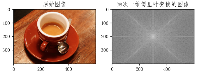

② Translation: Shifting f(x,y) in space corresponds to multiplying its Fourier transform by an exponential factor. ③ Rotation: Rotating f(x,y) by an angle results in the same rotation of its Fourier transform F(u,v).

3 Fast Fourier Transform

• The discrete Fourier transform (DFT) is a crucial tool in digital signal processing, but its high computational demand and long processing time have limited its widespread use.
• The fast Fourier transform (FFT) significantly improves computational speed, enabling real-time processing in certain applications and making it suitable for control systems.
• The FFT is not a new transform but an efficient algorithm for computing the DFT by eliminating redundant calculations.

3.1 Principle of Fast Fourier Transform

• The computational time of DFT is primarily determined by the number of multiplications. The FFT reduces this by decomposing the calculation and exploiting periodicity.
• The key to achieving fast computation is reducing the number of multiplications through periodicity and decomposition.

3.2 Implementation of Fast Fourier Transform

• The basic idea of FFT is based on the successive doubling method, which breaks down the Fourier transform of 2M data points into two Fourier transforms of M data points each, reducing the computational complexity from 4*M*M to 2*M*M.
• This process can be recursively applied until only small groups of data points remain.

4 Frequency Domain Filtering of Images

• Image transformation redistributes energy to facilitate processing, such as noise removal and feature enhancement.
• Fourier transform has significant applications in image analysis, filtering, enhancement, and compression.
• Assuming the original image f(x,y) is transformed to F(u,v), frequency domain enhancement involves adjusting the frequency components using a filter function H(u,v), then applying the inverse transform to obtain the enhanced image g(x,y).
• Suitable filter functions can be designed to emphasize specific features of the image. For example, highlighting high-frequency components enhances edges (high-pass filtering), while emphasizing low-frequency components smooths the image (low-pass filtering).
• The basic steps for frequency domain filtering are: (1) Transform the original image f(x,y) to F(u,v) using FFT; (2) Convolve F(u,v) with the filter function H(u,v) to get G(u,v); (3) Apply inverse FFT to G(u,v) to obtain the enhanced image g(x,y).

4.1 Low-pass Filtering

• In the frequency domain, low-frequency components correspond to regions with gradual gray value changes, while high-frequency components represent edges and noise.
• Low-pass filtering preserves low-frequency components while attenuating high-frequency components using a filter function H(u,v), similar to spatial domain smoothing filters that reduce noise and smooth images.

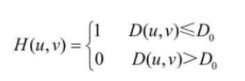
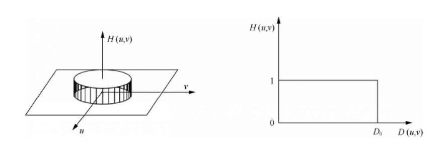
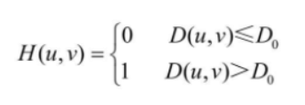
First Type: Ideal Low-pass Filter

• The transfer function of a two-dimensional ideal low-pass filter is defined as:
• Ideal low-pass filter and its image

from matplotlib import pyplot as plt
import numpy as np
from skimage import data, color

# Function to enable Chinese font display
def set_ch():
    from pylab import mpl
    mpl.rcParams['font.sans-serif'] = ['FangSong']
    mpl.rcParams['axes.unicode_minus'] = False

set_ch()
D = 10
new_img = data.coffee()
new_img = color.rgb2gray(new_img)
# Fourier transform
f1 = np.fft.fft2(new_img)
# Shift the center point to the middle
f1_shift = np.fft.fftshift(f1)
# Implement ideal low-pass filter
rows, cols = new_img.shape
crow, ccol = int(rows / 2), int(cols / 2)  # Calculate spectrum center
mask = np.zeros((rows, cols), dtype='uint8')  # Create a matrix of zeros
# Set low-pass components within distance D from the center to 1
for i in range(rows):
    for j in range(cols):
        if np.sqrt(i * i + j * j) <= D:
            mask[crow - D:crow + D, ccol - D:ccol + D] = 1
f1_shift = f1_shift * mask
# Inverse Fourier transform
f_ishift = np.fft.ifftshift(f1_shift)
img_back = np.fft.ifft2(f_ishift)
img_back = np.abs(img_back)
img_back = (img_back - np.amin(img_back)) / (np.amax(img_back) - np.amin(img_back))

plt.figure()
plt.subplot(121)
plt.imshow(new_img, cmap='gray')
plt.title('Original Image')

plt.subplot(122)
plt.imshow(img_back, cmap='gray')
plt.title('Filtered Image')
plt.show()

• Two-dimensional image ideal low-pass filtering

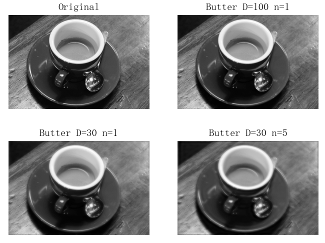
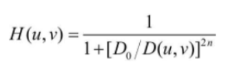
Second Type: Butterworth Low-pass Filter

• The transfer function of a Butterworth low-pass filter is defined as:
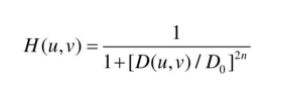
• D0 is the cutoff frequency, and n is the order of the filter. Typically, D0 is chosen as the distance where the maximum value of H(u,v) drops to half.
• Butterworth low-pass filter cross-section
• Compared to the ideal low-pass filter, the Butterworth filter has smoother transitions between high and low frequencies, reducing the ringing effect.
• With lower order n, the transition is smoother. As n increases, the ringing effect becomes more pronounced.

from matplotlib import pyplot as plt
import numpy as np
from skimage import data, color

# Function to enable Chinese font display
def set_ch():
    from pylab import mpl
    mpl.rcParams['font.sans-serif'] = ['FangSong']
    mpl.rcParams['axes.unicode_minus'] = False

set_ch()
img = data.coffee()
img = color.rgb2gray(img)
f = np.fft.fft2(img)
fshift = np.fft.fftshift(f)
# Convert to absolute values and apply logarithm for visualization
s1 = np.log(np.abs(fshift))

def ButterworthPassFilter(image, d, n):
    """
    Butterworth low-pass filter
    """
    f = np.fft.fft2(image)
    fshift = np.fft.fftshift(f)

    def make_transform_matrix(d):
        transform_matrix = np.zeros(image.shape)
        center_point = tuple(map(lambda x: (x - 1) / 2, s1.shape))
        for i in range(transform_matrix.shape[0]):
            for j in range(transform_matrix.shape[1]):
                def cal_distance(pa, pb):
                    from math import sqrt
                    dis = sqrt((pa[0] - pb[0]) ** 2 + (pa[1] - pb[1]) ** 2)
                    return dis

                dis = cal_distance(center_point, (i, j))
                transform_matrix[i, j] = 1 / (1 + (dis / d) ** (2 * n))
        return transform_matrix

    d_matrix = make_transform_matrix(d)
    new_img = np.abs(np.fft.ifft2(np.fft.ifftshift(fshift * d_matrix)))
    return new_img


plt.subplot(221)
plt.axis('off')
plt.title('Original')
plt.imshow(img, cmap='gray')

plt.subplot(222)
plt.axis('off')
plt.title('Butter D=100 n=1')
butter_100_1 = ButterworthPassFilter(img, 100, 1)
plt.imshow(butter_100_1, cmap='gray')

plt.subplot(223)
plt.axis('off')
plt.title('Butter D=30 n=1')
butter_30_1 = ButterworthPassFilter(img, 30, 1)
plt.imshow(butter_30_1, cmap='gray')

plt.subplot(224)
plt.axis('off')
plt.title('Butter D=30 n=5')
butter_30_5 = ButterworthPassFilter(img, 30, 5)
plt.imshow(butter_30_5, cmap='gray')

plt.show()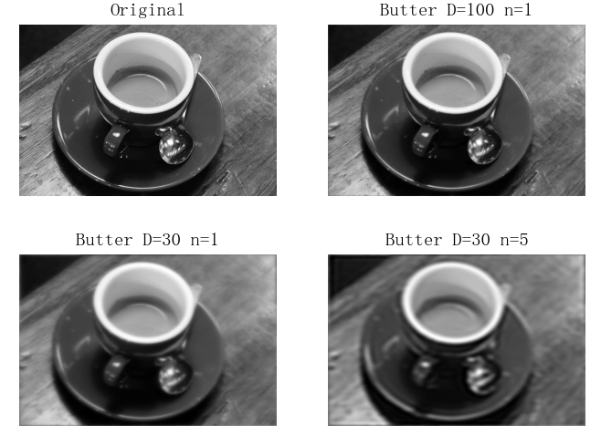

4.2 High-pass Filtering

• Image edges and details are primarily in the high-frequency components, while blurring is caused by weak high-frequency components.
• High-pass filtering suppresses low-frequency components to enhance high-frequency components, making edges and lines clearer and sharpening the image.

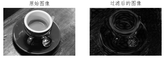
First Type: Ideal High-pass Filter

• The ideal high-pass filter has a transfer function that is the opposite of the ideal low-pass filter.
• Ideal high-pass filter and its image

from matplotlib import pyplot as plt
import numpy as np
from skimage import data, color

# Function to enable Chinese font display
def set_ch():
    from pylab import mpl
    mpl.rcParams['font.sans-serif'] = ['FangSong']
    mpl.rcParams['axes.unicode_minus'] = False

set_ch()
D = 10
new_img = data.coffee()
new_img = color.rgb2gray(new_img)
# Fourier transform
f1 = np.fft.fft2(new_img)
f1_shift = np.fft.fftshift(f1)
"""
Implement ideal high-pass filter
"""
rows, cols = new_img.shape
# Calculate spectrum center
crow, ccol = int(rows / 2), int(cols / 2)
# Create a matrix of zeros
mask = np.zeros((rows, cols), dtype='uint8')
# Set low-pass components within distance D from the center to 1
for i in range(rows):
    for j in range(cols):
        if np.sqrt(i * i + j * j) <= D:
            mask[crow - D:crow + D, ccol - D:ccol + D] = 1

mask = 1 - mask
f1_shift = f1_shift * mask
"""
End of ideal high-pass filter implementation
"""
# Inverse Fourier transform
f_ishift = np.fft.ifftshift(f1_shift)
img_back = np.fft.ifft2(f_ishift)
img_back = np.abs(img_back)
img_back = (img_back - np.amin(img_back)) / (np.amax(img_back) - np.amin(img_back))

plt.figure()
plt.subplot(121)
plt.axis('off')
plt.imshow(new_img, cmap='gray')
plt.title('Original Image')

plt.subplot(122)
plt.axis('off')
plt.imshow(img_back, cmap='gray')
plt.title('Filtered Image')
plt.show()

• Two-dimensional image ideal high-pass filtering

Second Type: Butterworth High-pass Filter

• The Butterworth high-pass filter has a transfer function that is the opposite of the Butterworth low-pass filter, providing smoother transitions and reducing ringing effects.

from matplotlib import pyplot as plt
import numpy as np
from skimage import data, color

# Function to enable Chinese font display
def set_ch():
    from pylab import mpl
    mpl.rcParams['font.sans-serif'] = ['FangSong']
    mpl.rcParams['axes.unicode_minus'] = False

set_ch()
img = data.coffee()
img = color.rgb2gray(img)
f = np.fft.fft2(img)
fshift = np.fft.fftshift(f)
# Convert to absolute values and apply logarithm for visualization
s1 = np.log(np.abs(fshift))

def ButterworthPassFilter(image, d, n):
    """
    Butterworth high-pass filter
    """
    f = np.fft.fft2(image)
    fshift = np.fft.fftshift(f)

    def make_transform_matrix(d):
        transform_matrix = np.zeros(image.shape)
        center_point = tuple(map(lambda x: (x - 1) / 2, s1.shape))
        for i in range(transform_matrix.shape[0]):
            for j in range(transform_matrix.shape[1]):
                def cal_distance(pa, pb):
                    from math import sqrt
                    dis = sqrt((pa[0] - pb[0]) ** 2 + (pa[1] - pb[1]) ** 2)
                    return dis

                dis = cal_distance(center_point, (i, j))
                transform_matrix[i, j] = 1 / (1 + (dis / d) ** (2 * n))
        return transform_matrix

    d_matrix = make_transform_matrix(d)
    d_matrix = 1 - d_matrix
    new_img = np.abs(np.fft.ifft2(np.fft.ifftshift(fshift * d_matrix)))
    return new_img


plt.subplot(221)
plt.axis('off')
plt.title('Original')
plt.imshow(img, cmap='gray')

plt.subplot(222)
plt.axis('off')
plt.title('Butter D=100 n=1')
butter_100_1 = ButterworthPassFilter(img, 100, 1)
plt.imshow(butter_100_1, cmap='gray')

plt.subplot(223)
plt.axis('off')
plt.title('Butter D=30 n=1')
butter_30_1 = ButterworthPassFilter(img, 30, 1)
plt.imshow(butter_30_1, cmap='gray')

plt.subplot(224)
plt.axis('off')
plt.title('Butter D=30 n=5')
butter_30_5 = ButterworthPassFilter(img, 30, 5)
plt.imshow(butter_30_5, cmap='gray')

plt.show()

Third Type: High-frequency Enhancement Filter

• High-pass filtering removes low-frequency components, making edges stronger but causing smooth regions to become dark.
• High-frequency enhancement filters add a constant to the high-pass filter transfer function, preserving some low-frequency components to maintain gray level details while improving edge contrast.
• The transfer function is He(u,v) = k*H(u,v) + c.

from matplotlib import pyplot as plt
import numpy as np
from skimage import data, color

# Function to enable Chinese font display
def set_ch():
    from pylab import mpl
    mpl.rcParams['font.sans-serif'] = ['FangSong']
    mpl.rcParams['axes.unicode_minus'] = False

set_ch()
img = data.coffee()
img = color.rgb2gray(img)
f = np.fft.fft2(img)
fshift = np.fft.fftshift(f)
# Convert to absolute values and apply logarithm for visualization
s1 = np.log(np.abs(fshift))

def ButterworthPassFilter(image, d, n):
    """
    Butterworth high-pass filter
    """
    f = np.fft.fft2(image)
    fshift = np.fft.fftshift(f)

    def make_transform_matrix(d):
        transform_matrix = np.zeros(image.shape)
        center_point = tuple(map(lambda x: (x - 1) / 2, s1.shape))
        for i in range(transform_matrix.shape[0]):
            for j in range(transform_matrix.shape[1]):
                def cal_distance(pa, pb):
                    from math import sqrt
                    dis = sqrt((pa[0] - pb[0]) ** 2 + (pa[1] - pb[1]) ** 2)
                    return dis

                dis = cal_distance(center_point, (i, j))
                transform_matrix[i, j] = 1 / (1 + (dis / d) ** (2 * n))
        return transform_matrix

    d_matrix = make_transform_matrix(d)
    d_matrix = d_matrix + 0.5
    new_img = np.abs(np.fft.ifft2(np.fft.ifftshift(fshift * d_matrix)))
    return new_img


plt.subplot(221)
plt.axis('off')
plt.title('Original')
plt.imshow(img, cmap='gray')

plt.subplot(222)
plt.axis('off')
plt.title('Butter D=100 n=1')
butter_100_1 = ButterworthPassFilter(img, 100, 1)
plt.imshow(butter_100_1, cmap='gray')

plt.subplot(223)
plt.axis('off')
plt.title('Butter D=30 n=1')
butter_30_1 = ButterworthPassFilter(img, 30, 1)
plt.imshow(butter_30_1, cmap='gray')

plt.subplot(224)
plt.axis('off')
plt.title('Butter D=30 n=5')
butter_30_5 = ButterworthPassFilter(img, 30, 5)
plt.imshow(butter_30_5, cmap='gray')

plt.show()

• Two-dimensional image high-frequency enhancement filtering results