Image Feature Extraction

Image features are a series of mathematical sets that can represent the content or characteristics of an image, including natural features (such as brightness, color, texture) and artificial features (such as image spectrum, image histogram). Image feature extraction transforms images from their original attribute space to a feature attribute space. This process involves analyzing image information to extract features less susceptible to random factors, converting the original image features into ones with clear physical or statistical meanings. After feature extraction, feature selection often follows to remove redundant information, improving recognition accuracy, reducing computational workload, and increasing processing speed. Good image features should have representativeness or distinguishability, stability, and independence.

Image feature extraction can be categorized into low-level feature extraction (focusing on color, texture, shape) and high-level semantic feature extraction (focusing on semantic layers like human recognition). It can also be divided into global feature extraction (focusing on overall image representation) and local feature extraction (focusing on specific local regions).

1. Image Color Feature Extraction

Color features are simple yet widely used visual features, less dependent on image size, direction, and viewpoint. They are global features describing the surface properties of objects in an image.

1.1 Color Histogram

A color histogram describes the distribution of pixel colors in an image, showing color statistics and dominant tones but not spatial information.

from matplotlib import pyplot as plt
from skimage import data, exposure

def set_ch():
    from pylab import mpl
    mpl.rcParams['font.sans-serif'] = ['FangSong']
    mpl.rcParams['axes.unicode_minus'] = False

set_ch()
img = data.coffee()

plt.figure()
plt.subplot(221)
plt.axis('off')
plt.title('Original Image')
plt.imshow(img)

plt.subplot(222)
plt.axis('off')
plt.title('R Channel Histogram')
plt.hist(img[:, :, 0].ravel(), bins=256, color='red', alpha=0.6)

plt.subplot(223)
plt.axis('off')
plt.title('G Channel Histogram')
plt.hist(img[:, :, 1].ravel(), bins=256, color='green', alpha=0.6)

plt.subplot(224)
plt.axis('off')
plt.title('B Channel Histogram')
plt.hist(img[:, :, 2].ravel(), bins=256, color='blue', alpha=0.6)
plt.show()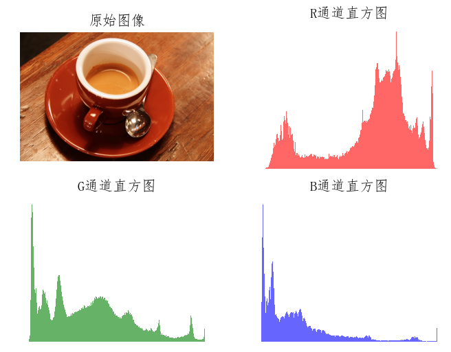

1.2 Color Moments

Color moments represent color distribution using the first three moments (mean, variance, skewness) for each color channel.

from matplotlib import pyplot as plt
from skimage import data, exposure
import numpy as np
from scipy import stats

def set_ch():
    from pylab import mpl
    mpl.rcParams['font.sans-serif'] = ['FangSong']
    mpl.rcParams['axes.unicode_minus'] = False

set_ch()

image = data.coffee()
features = np.zeros(shape=(3, 3))
for k in range(image.shape[2]):
    mu = np.mean(image[:, :, k])
    delta = np.std(image[:, :, k])
    skew = np.mean(stats.skew(image[:, :, k]))
    features[0, k] = mu
    features[1, k] = delta
    features[2, k] = skew
print(features)

1.3 Color Set

A color set approximates a color histogram by quantizing color space and using automatic segmentation techniques.

1.4 Color Coherence Vector

A color coherence vector extends color histogram information by distinguishing between coherent and non-coherent pixels based on region size thresholds.

1.5 Color Correlogram

A color correlogram describes spatial relationships between color pairs using relative distance distributions.

from matplotlib import pyplot as plt
from skimage import data, exposure
import numpy as np
from scipy import stats

def set_ch():
    from pylab import mpl
    mpl.rcParams['font.sans-serif'] = ['FangSong']
    mpl.rcParams['axes.unicode_minus'] = False

set_ch()

def isValid(X, Y, point):
    if point[0] < 0 or point[0] >= X:
        return False
    if point[1] < 0 or point[1] >= Y:
        return False
    return True

def getNeighbors(X, Y, x, y, dist):
    cn1 = (x + dist, y + dist)
    cn2 = (x + dist, y)
    cn3 = (x + dist, y - dist)
    cn4 = (x, y - dist)
    cn5 = (x - dist, y - dist)
    cn6 = (x - dist, y)
    cn7 = (x - dist, y + dist)
    cn8 = (x, y + dist)
    points = (cn1, cn2, cn3, cn4, cn5, cn6, cn7, cn8)
    Cn = []
    for i in points:
        if isValid(X, Y, i):
            Cn.append(i)
    return Cn

def corrlogram(image, dist):
    XX, YY, tt = image.shape
    cgram = np.zeros((256, 256), dtype=np.int)
    for x in range(XX):
        for y in range(YY):
            for t in range(tt):
                color_i = image[x, y, t]
                neighbors_i = getNeighbors(XX, YY, x, y, dist)
                for j in neighbors_i:
                    j0 = j[0]
                    j1 = j[1]
                    color_j = image[j0, j1, t]
                    cgram[color_i, color_j] += 1
    return cgram

img = data.coffee()
dist = 4
cgram = corrlogram(img, dist)
plt.imshow(cgram)
plt.show()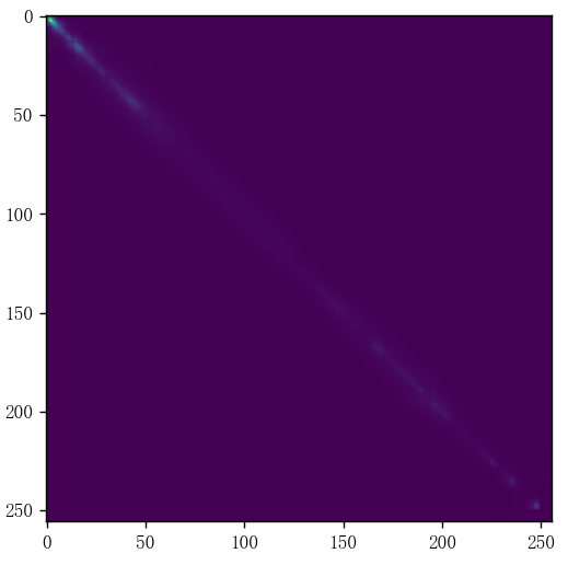

2. Image Texture Feature Extraction

Texture reflects the visual characteristics of homogeneous phenomena in images, showing regularity, periodicity, and homogeneity. Texture features describe surface properties of objects but not their essential attributes.

2.1 Statistical Texture Analysis Methods

Statistical methods describe textures through spatial frequency, boundary frequency, and gray-level dependencies.

from matplotlib import pyplot as plt
from skimage.feature import greycomatrix, greycoprops
from skimage import data
import numpy as np

def set_ch():
    from pylab import mpl
    mpl.rcParams['font.sans-serif'] = ['FangSong']
    mpl.rcParams['axes.unicode_minus'] = False

set_ch()
PATCH_SIZE = 21
image = data.camera()
grass_locations = [(474, 291), (440, 433), (466, 18), (462, 236)]
grass_patches = []
for loc in grass_locations:
    grass_patches.append(image[loc[0]:loc[0]+PATCH_SIZE, loc[1]:loc[1]+PATCH_SIZE])

sky_locations = [(54, 48), (21, 233), (90, 380), (195, 330)]
sky_patches = []
for loc in sky_locations:
    sky_patches.append(image[loc[0]:loc[0]+PATCH_SIZE, loc[1]:loc[1]+PATCH_SIZE])

xs = []
ys = []
for patch in (grass_patches + sky_patches):
    glcm = greycomatrix(patch, [5], [0], 256, symmetric=True, normed=True)
    xs.append(greycoprops(glcm, 'dissimilarity')[0, 0])
    ys.append(greycoprops(glcm, 'correlation')[0, 0])

fig = plt.figure(figsize=(8, 8))
ax = fig.add_subplot(3, 2, 1)
ax.imshow(image, cmap=plt.cm.gray, interpolation='nearest', vmin=0, vmax=255)
for (y, x) in grass_locations:
    ax.plot(x + PATCH_SIZE/2, y + PATCH_SIZE/2, 'gs')
for (y, x) in sky_locations:
    ax.plot(x + PATCH_SIZE/2, y + PATCH_SIZE, 'bs')
ax.set_xlabel('Original Image')
ax.set_xticks([])
ax.set_yticks([])
ax.axis('image')

ax = fig.add_subplot(3, 2, 2)
ax.plot(xs[:len(grass_patches)], ys[:len(grass_patches)], 'go', label='Grass')
ax.plot(xs[:len(sky_patches)], ys[:len(sky_patches)], 'bo', label='Sky')
ax.set_xlabel('GLCM Dissimilarity')
ax.set_ylabel('GLCM Correlation')
ax.legend()

for i, patch in enumerate(grass_patches):
    ax = fig.add_subplot(3, len(grass_patches), len(grass_patches)*1 + i + 1)
    ax.imshow(patch, cmap=plt.cm.gray, interpolation='nearest', vmin=0, vmax=255)
    ax.set_xlabel('Grass %d' % (i + 1))

for i, patch in enumerate(sky_patches):
    ax = fig.add_subplot(3, len(sky_patches), len(sky_patches)*2 + i + 1)
    ax.imshow(patch, cmap=plt.cm.gray, interpolation='nearest', vmin=0, vmax=255)
    ax.set_xlabel('Sky %d' % (i + 1))

fig.suptitle('Grey level co-occurrence matrix features', fontsize=14)
plt.show()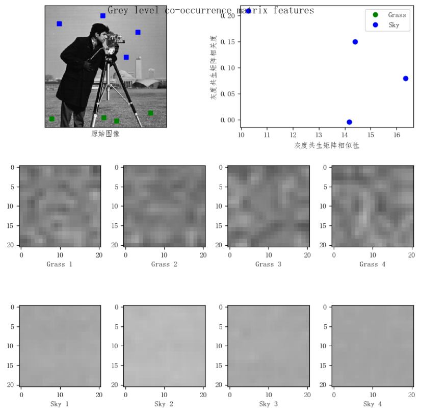

2.2 Laws Texture Energy Measurement

Laws' texture energy measurement uses micro-window filtering and macro-window energy transformation to extract texture features.

2.3 Gabor Transform

Gabor transform decomposes images using filters with different frequencies and orientations, inspired by human visual processing.

2.4 Local Binary Pattern

Local Binary Pattern (LBP) encodes local texture by comparing neighborhood pixel values to a center pixel threshold.

import skimage.feature
import skimage.segmentation
import skimage.data
import matplotlib.pyplot as plt

def set_ch():
    from pylab import mpl
    mpl.rcParams['font.sans-serif'] = ['FangSong']
    mpl.rcParams['axes.unicode_minus'] = False

set_ch()
img = skimage.data.coffee()
for colour_channel in (0, 1, 2):
    img[:, :, colour_channel] = skimage.feature.local_binary_pattern(img[:, :, colour_channel], 8, 1.0, method='var')
plt.imshow(img)
plt.show()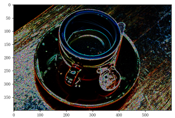

3. Image Shape Feature Extraction

Shape features require object or region segmentation in images and can be contour-based (like Fourier descriptors) or region-based (like shape invariants).

3.1 Simple Shape Features

• Rectangularity: Ratio of object area to minimum bounding rectangle area.
• Sphericity: Describes how spherical an object is.
• Circularity: Defined by boundary points of a region.

3.2 Fourier Descriptors

Fourier descriptors represent closed curves using Fourier coefficients from coordinate sequences.

3.3 Shape Invariants

Shape invariants remain unchanged under geometric transformations like translation, rotation, and scaling, aiding object classification.

4. Image Edge Feature Extraction

Edges have direction and magnitude, detected through image derivatives. The process involves filtering, enhancing, detecting, and localizing edges.

4.1 Gradient Edge Detection

Edges are found where gradient magnitude exceeds a threshold, indicating rapid intensity changes.

4.2 First-Order Edge Detection Operators

Roberts Operator

Roberts operator detects edges using diagonal pixel differences.

import matplotlib.pyplot as plt
from skimage.data import camera
from skimage.filters import roberts

def set_ch():
    from pylab import mpl
    mpl.rcParams['font.sans-serif'] = ['FangSong']
    mpl.rcParams['axes.unicode_minus'] = False

set_ch()
image = camera()
edge_roberts = roberts(image)
fig, ax = plt.subplots(ncols=2, sharex=True, sharey=True, figsize=(8, 4))
ax[0].imshow(image, cmap='gray')
ax[0].set_title('Original Image')
ax[1].imshow(edge_roberts, cmap='gray')
ax[1].set_title('Roberts Edge Detection')
for a in ax:
    a.axis('off')
plt.tight_layout()
plt.show()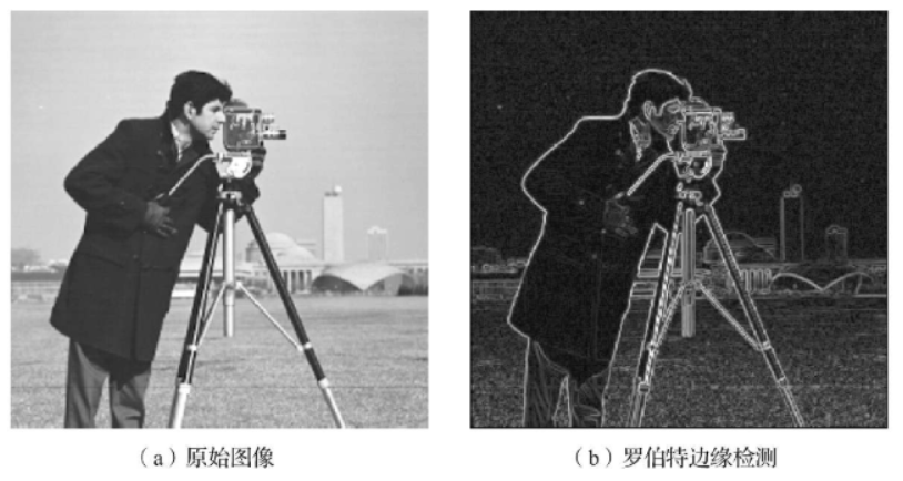

Sobel Operator

Sobel operator calculates gradient magnitude using two kernels, providing edge detection with some noise reduction.

import matplotlib.pyplot as plt
from skimage.data import camera
from skimage.filters import sobel, sobel_v, sobel_h

def set_ch():
    from pylab import mpl
    mpl.rcParams['font.sans-serif'] = ['FangSong']
    mpl.rcParams['axes.unicode_minus'] = False

set_ch()
image = camera()
edge_sobel = sobel(image)
edge_sobel_v = sobel_v(image)
edge_sobel_h = sobel_h(image)
fig, ax = plt.subplots(ncols=2, nrows=2, sharex=True, sharey=True, figsize=(8, 4))
ax[0, 0].imshow(image, cmap=plt.cm.gray)
ax[0, 0].set_title('Original Image')
ax[0, 1].imshow(edge_sobel, cmap=plt.cm.gray)
ax[0, 1].set_title('Sobel Edge Detection')
ax[1, 0].imshow(edge_sobel_v, cmap=plt.cm.gray)
ax[1, 0].set_title('Sobel Vertical Edge Detection')
ax[1, 1].imshow(edge_sobel_h, cmap=plt.cm.gray)
ax[1, 1].set_title('Sobel Horizontal Edge Detection')
for a in ax:
    for j in a:
        j.axis('off')
plt.tight_layout()
plt.show()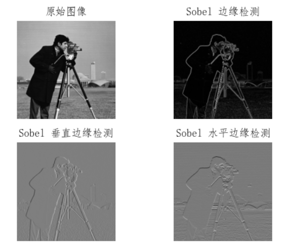

Prewitt Operator

Prewitt operator, similar to Sobel but with simpler coefficients, detects edges using gradient calculations.

4.3 Second-Order Edge Detection Operators

Laplacian Operator

Laplacian operator detects edges by finding zero crossings in the second derivative.

import matplotlib.pyplot as plt
from skimage.data import camera, coffee
from skimage.filters import laplace

def set_ch():
    from pylab import mpl
    mpl.rcParams['font.sans-serif'] = ['FangSong']
    mpl.rcParams['axes.unicode_minus'] = False

set_ch()
image_camera = camera()
edge_laplace_camera = laplace(image_camera)
image_coffee = coffee()
edge_laplace_coffee = laplace(image_coffee)
fig, ax = plt.subplots(ncols=2, nrows=2, sharex=True, sharey=True, figsize=(8, 6))
ax[0, 0].imshow(image_camera, cmap=plt.cm.gray)
ax[0, 0].set_title('Original Image')
ax[0, 1].imshow(edge_laplace_camera, cmap=plt.cm.gray)
ax[0, 1].set_title('Laplace Edge Detection')
ax[1, 0].imshow(image_coffee, cmap=plt.cm.gray)
ax[1, 0].set_title('Original Image')
ax[1, 1].imshow(edge_laplace_coffee, cmap=plt.cm.gray)
ax[1, 1].set_title('Laplace Edge Detection')
for a in ax:
    for j in a:
        j.axis('off')
plt.tight_layout()
plt.show()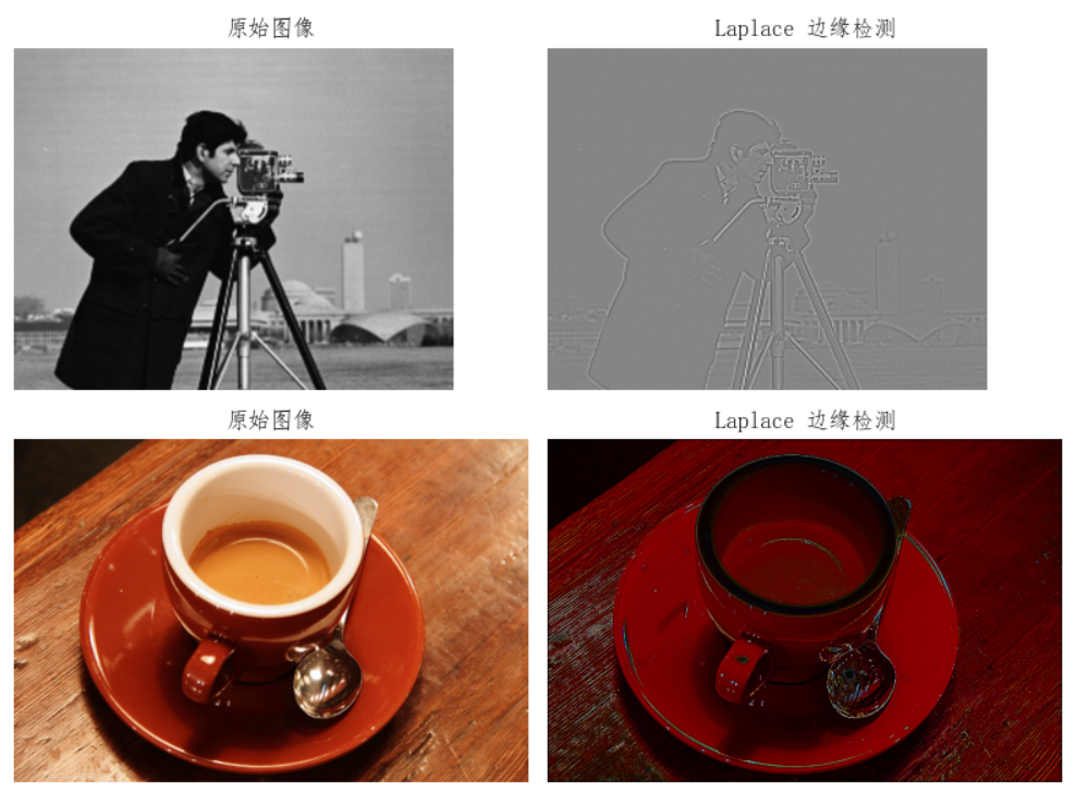

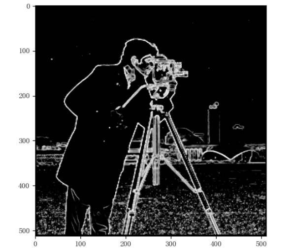
LoG Operator

LoG (Laplacian of Gaussian) operator combines Gaussian smoothing with Laplacian edge detection to reduce noise impact.

import matplotlib.pyplot as plt
from skimage.data import camera, coffee
from skimage.filters import laplace, gaussian

def set_ch():
    from pylab import mpl
    mpl.rcParams['font.sans-serif'] = ['FangSong']
    mpl.rcParams['axes.unicode_minus'] = False

set_ch()
image = camera()
edge_laplace = laplace(image)
gaussian_image = gaussian(image)
edge_LoG = laplace(gaussian_image)
fig, ax = plt.subplots(ncols=2, nrows=2, sharex=True, sharey=True, figsize=(8, 6))
ax[0, 0].imshow(image, cmap=plt.cm.gray)
ax[0, 0].set_title('Original Image')
ax[0, 1].imshow(edge_laplace, cmap=plt.cm.gray)
ax[0, 1].set_title('Laplace Edge Detection')
ax[1, 0].imshow(gaussian_image, cmap=plt.cm.gray)
ax[1, 0].set_title('Gaussian Smoothed Image')
ax[1, 1].imshow(edge_LoG, cmap=plt.cm.gray)
ax[1, 1].set_title('LoG Edge Detection')
for a in ax:
    for j in a:
        j.axis('off')
plt.tight_layout()
plt.show()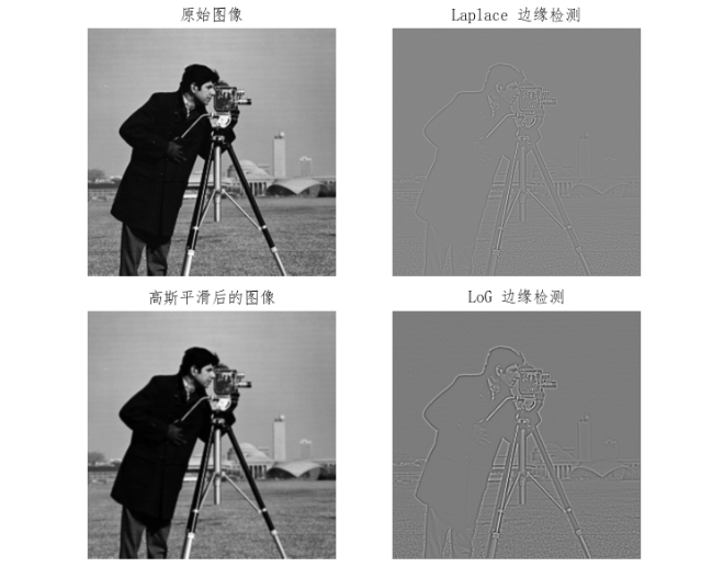

5. Image Point Feature Extraction

Point features, like corners, are small regions with distinct intensity changes. Corner detection is widely studied and applied.

5.1 SUSAN Corner Detection

SUSAN (Smallest Univalue Segment Assimilating Nucleus) detects corners by analyzing intensity similarity in a circular neighborhood.

import matplotlib.pyplot as plt
from skimage.data import camera
import numpy as np

def set_ch():
    from pylab import mpl
    mpl.rcParams['font.sans-serif'] = ['FangSong']
    mpl.rcParams['axes.unicode_minus'] = False

def susan_mask():
    mask = np.ones((7, 7))
    mask[0, 0] = 0
    mask[0, 1] = 0
    mask[0, 5] = 0
    mask[0, 6] = 0
    mask[1, 0] = 0
    mask[1, 6] = 0
    mask[5, 0] = 0
    mask[5, 6] = 0
    mask[6, 0] = 0
    mask[6, 1] = 0
    mask[6, 5] = 0
    mask[6, 6] = 0
    return mask

def susan_corner_detection(img):
    img = img.astype(np.float64)
    g = 37 / 2
    circularMask = susan_mask()
    output = np.zeros(img.shape)
    for i in range(3, img.shape[0] - 3):
        for j in range(3, img.shape[1] - 3):
            ir = np.array(img[i-3:i+4, j-3:j+4])
            ir = ir[circularMask == 1]
            ir0 = img[i, j]
            a = np.sum(np.exp(-((ir - ir0) / 10) ** 6))
            if a <= g:
                a = g - a
            else:
                a = 0
            output[i, j] = a
    return output

set_ch()
image = camera()
out = susan_corner_detection(image)
plt.imshow(out, cmap='gray')
plt.show()