Image Compression

After digitization, image data can occupy a large amount of space. For example, a 32-bit grayscale image with a resolution of 800x600 pixels has 480,000 pixels and occupies 480,000 x 32 bits = 480,000 x 4B = 1.83MB. Storing one second of film at this resolution would require 1.83 x 24 = 43.92MB. The large size of image data creates difficulties for storage and transmission, making image compression necessary to remove redundant information and achieve effective compression.

1 Introduction to Image Compression

Data represents information, and if different methods use different information to represent the same quantity, some information in the more data-intensive method is likely useless. The existence of redundant data makes image compression possible.

1.1 Types of Redundancy

• Coding Redundancy : If more coding symbols than necessary are used to represent the grayscale levels of an image, the image has coding redundancy. For example, using 8 bits instead of 1 bit to represent a pixel introduces redundancy.
• Pixel Intensity Redundancy : Pixel values in an image are not entirely random but are related to adjacent pixels. Many individual pixels contribute redundantly to visual perception and can be predicted from neighboring pixels, reducing the information each pixel carries. For instance, the original image data 234 223 231 238 235 can be compressed to 234 -11 8 7 -3.
• Psycho-visual Redundancy : The eye's sensitivity to visual information varies, and some information is less important in typical visual processing. Removing this information doesn't significantly degrade image quality.

1.2 Compression Algorithm Categories

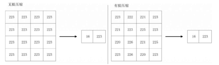
Image compression algorithms are based on coding, pixel intensity, and psycho-visual redundancy. They are broadly classified into lossless and lossy compression.

• Lossless Compression Methods : Include run-length encoding and entropy encoding, allowing complete recovery of the original information after compression.
• Lossy Compression Methods : Include transform encoding and fractal compression, which cause some information loss that prevents full reconstruction of the original image.

Common encoding methods include:

• Entropy Encoding or Statistical Encoding : Assigns shorter codes to more probable symbols and longer codes to less probable ones, minimizing average code length. Main methods include Huffman, Shannon, and arithmetic encoding.
• Predictive Encoding : Uses adjacent known pixels (or blocks) to predict current pixel (or block) values, then quantizes and encodes the prediction error. Includes PCM and DPCM.
• Transform Encoding : Transforms spatial domain images to another orthogonal vector space, producing transform coefficients for encoding.
• Hybrid Encoding : Combines entropy, transform, or predictive encoding methods, as in JPEG and MPEG standards.

2 Entropy Encoding Techniques

Entropy encoding is a lossless technique based on information theory, assigning shorter codes to more probable symbols and longer codes to less probable ones to minimize average code length. Main methods include Huffman, Shannon, and arithmetic encoding. Information entropy represents the optimal encoding length for a data set or sequence, with various entropy encoding algorithms approximating this theoretical value.

2.1 Huffman Encoding

Huffman encoding is a variable-length encoding method. It scans image data to calculate pixel probabilities, assigns unique code words based on these probabilities, and creates a Huffman table. The encoded image records pixel code words, with the code-word to pixel value mapping stored in the table.

Basic Steps of Huffman Encoding :

1. Sort pixel values by probability and combine the two lowest-probability symbols.
2. Encode the simplified pixels, starting from the lowest-probability symbol and proceeding to all elements.

import numpy as np
import queue

# Define the image to be encoded
image = np.array([[3, 1, 2, 4], [2, 4, 0, 2], [2, 2, 3, 3], [2, 4, 4, 2]])
# Calculate the probability of each element
hist = np.bincount(image.ravel(), minlength=5)
probabilities = hist / np.sum(hist)

# Find the smallest element in the data
def get_smallest(data):
    first = second = 1
    fid = sid = 0
    for idx, element in enumerate(data):
        if element < first:
            second = first
            sid = fid
            first = element
            fid = idx
        elif element < second and element != first:
            second = element
    return fid, first, sid, second

# Define the Huffman tree node
class Node:
    def __init__(self):
        self.prob = None
        self.code = None
        self.data = None
        self.left = None
        self.right = None

    def __lt__(self, other):
        if self.prob < other.prob:
            return 1
        else:
            return 0

    def __ge__(self, other):
        if self.prob > other.prob:
            return 1
        else:
            return 0

# Build the Huffman tree
def tree(probabilities):
    prq = queue.PriorityQueue()
    for color, probability in enumerate(probabilities):
        leaf = Node()
        leaf.data = color
        leaf.prob = probability
        prq.put(leaf)
    while prq.qsize() > 1:
        new_node = Node()
        l = prq.get()
        r = prq.get()
        new_node.left = l
        new_node.right = r
        new_prob = l.prob + r.prob
        new_node.prob = new_prob
        prq.put(new_node)
    return prq.get()

# Traverse the Huffman tree to derive codes
def huffman_traversal(root_node, tmp_array, f):
    if root_node.left is not None:
        tmp_array[huffman_traversal.count] = 1
        huffman_traversal.count += 1
        huffman_traversal(root_node.left, tmp_array, f)
        huffman_traversal.count -= 1
    if root_node.right is not None:
        tmp_array[huffman_traversal.count] = 0
        huffman_traversal.count += 1
        huffman_traversal(root_node.right, tmp_array, f)
        huffman_traversal.count -= 1
    else:
        huffman_traversal.output_bits[root_node.data] = huffman_traversal.count
        bit_stream = ''.join(str(cell) for cell in tmp_array[1:huffman_traversal.count])
        color = str(root_node.data)
        wr_str = color + '' + bit_stream + '\n'
        f.write(wr_str)
    return

root_node = tree(probabilities)
tmp_array = np.ones([4], dtype=int)
huffman_traversal.output_bits = np.empty(5, dtype=int)
huffman_traversal.count = 0
f = open('code.txt', 'w')
huffman_traversal(root_node, tmp_array, f)

Huffman encoding constructs data based on information theory, achieving near-optimal efficiency but with complexity in the encoding process.

2.2 Arithmetic Encoding

In arithmetic encoding, there's no one-to-one correspondence between source symbols and codes. Instead, an entire sequence of source symbols is assigned a real number interval between 0 and 1. As the sequence lengthens, the interval narrows, requiring more bits to represent it. Unlike Huffman encoding, arithmetic encoding can yield fractional average code lengths per symbol.

The arithmetic encoding process involves:

1. For a set of source symbols sorted by probability, set the current interval to [0,1). Divide this interval proportionally according to the symbol probabilities.
2. For each symbol in the input sequence, find its proportional sub-interval within the current interval, update the current interval to this sub-interval, and append the starting point of the new interval to the output.
3. Repeat the division and updating for the next symbol until the entire sequence is processed.
4. The final output is the encoded data representing the entire sequence.

Key considerations in arithmetic encoding include:

1. Limited computer precision can cause overflow, but this can be mitigated with scaling techniques.
2. Arithmetic encoders are highly sensitive to errors, which can corrupt the entire message.

Arithmetic encoding can be static or adaptive. Static encoding uses fixed symbol probabilities, while adaptive encoding dynamically updates probabilities based on symbol frequencies during encoding. The latter requires modeling to estimate source symbol probabilities during encoding.

2.3 Run-Length Encoding

Run-Length Encoding (RLE) is a Windows image file compression method that replaces sequences of identical adjacent pixels with a count and pixel value, reducing redundant bytes or bits. Decoding reverses this process, restoring the original data, making RLE a lossless technique. Its simplicity and speed make it effective for images with large uniform regions, such as bilevel images.

2.4 LZW Encoding

LZW is a lossless compression technique using a dynamically built translation table for repeated characters, suitable for data with high repetition. It involves three key objects: data stream, code stream, and string table. The algorithm extracts characters from the data, builds a string table, and replaces characters with table indices to reduce data size. The table is dynamically created during encoding and reconstructed during decoding.

string = 'abbababac'
dictionary = {'a': 1, 'b': 2, 'c': 3}
last = 4
p = ""
result = []
for c in string:
    pc = p + c
    if pc in dictionary:
        p = pc
    else:
        result.append(dictionary[p])
        dictionary[pc] = last
        last += 1
        p = c
if p != '':
    result.append(dictionary[p])
print(result)

3 Predictive Encoding

Predictive encoding leverages data correlations, using previous samples to predict new ones and reducing temporal/spatial redundancy. It encodes the difference between actual and predicted pixel values, eliminating redundancy. This method is lossy.

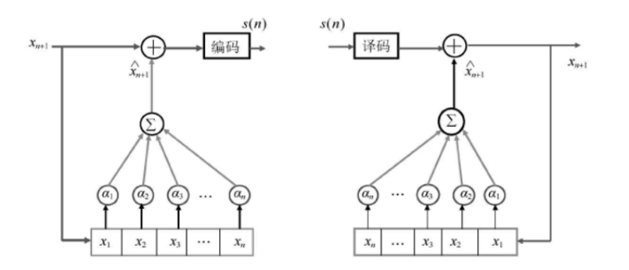
3.1 DPCM Encoding

Pulse Code Modulation (PCM) converts analog to digital signals, but directly storing images with PCM is data-intensive. DPCM instead predicts pixel values from previous ones, encodes the prediction error, and reduces data correlation.

DPCM Encoding Steps :

1. Read the image to be compressed.
2. Calculate the prediction error.
3. Quantize the error.

Decoder Process :

1. Receive quantized errors.
2. Calculate predicted values.
3. Add errors to predictions.

4 Transform Encoding

Transform encoding maps spatial domain images to another orthogonal space, producing transform coefficients. This reduces data correlation and redundancy, allowing for higher compression ratios when quantizing and encoding coefficients.

4.1 K-L Encoding

K-L transform (Hotelling transform) converts multi-band images into uncorrelated variables. The principal components have larger variances and contain most of the original information, making them useful for emphasizing image details.

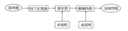
4.2 Discrete Cosine Transform

Discrete Cosine Transform (DCT) is widely used for signal and image compression. It concentrates signal energy in low-frequency components, offering de-correlation performance close to the K-L transform for Markov-like signals.

1. Blocking : Divide the input image into sub-blocks before DCT.
2. Transformation : Apply DCT to each row and column of each block to obtain a transform coefficient matrix.
3. Component Identification : The (0,0) element is the DC component, while others represent AC components of different frequencies.

5 JPEG Encoding

JPEG, developed by the Joint Picture Expert Group, is an international standard for static image compression. It defines three encoding systems:

1. A basic lossy system using DCT for most compression applications.
2. An extended system for high compression ratios and progressive reconstruction.
3. A lossless system for distortion-free applications.